Loading...
Contents
Top 50 Machine Learning Interview Questions
Sep 28, 202651 min read
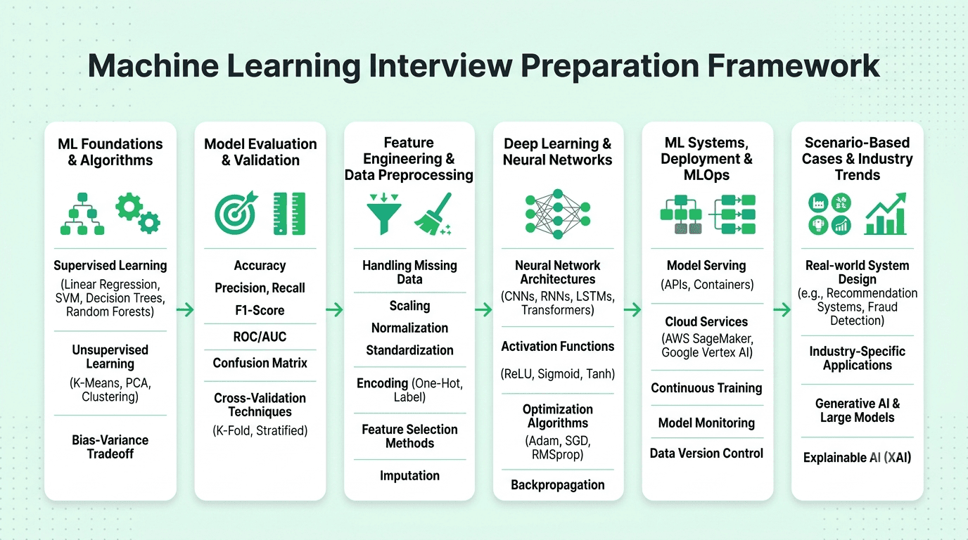
This guide covers the 50 most important machine learning interview questions, organized by topic and roughly ordered by frequency/importance within each category, moving from foundational learning theory through model evaluation, feature engineering, deep learning, ML systems/deployment, and current industry trends.
Categories:
ML Foundations: Learning Theory & Algorithms (Q1-10)
Model Evaluation & Validation (Q11-18)
Feature Engineering & Data Preprocessing (Q19-24)
Deep Learning & Neural Networks (Q25-32)
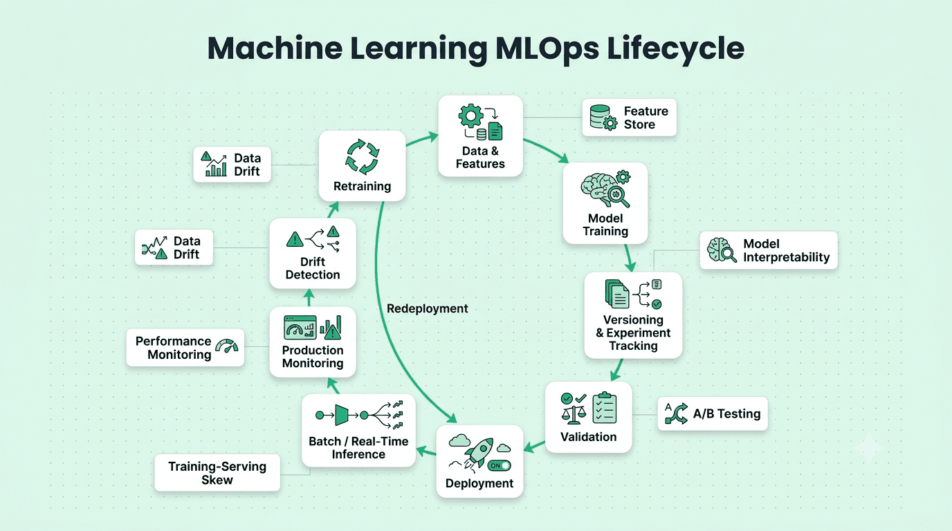
ML Systems, Deployment & MLOps (Q33-40)
Scenario-Based, Case Studies & Industry Trends (Q41-50)
FREE TO USE
25K+ INTERVIEWS4.8★ RATING68% IMPROVEMENT
Crack Your Dream Job
Real Interviews. Real Pressure. Practice until it feels easy.
- Seamless Interview Experience
- Resume & JD Questions
- Instant Personalized Feedback
Part 1: ML Foundations: Learning Theory & Algorithms
Question 1
Question: Explain the bias-variance tradeoff, and why it's central to machine learning model selection.
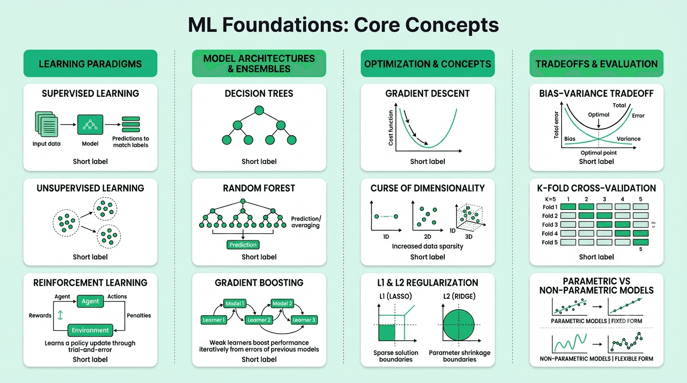
Answer: Bias is the error from overly simplistic model assumptions, causing systematic underfitting; variance is the error from excessive sensitivity to the specific training data, causing overfitting. Total expected error decomposes into bias squared, plus variance, plus irreducible noise — reducing one typically increases the other, and the goal of model selection is finding the complexity level that minimizes their combined effect on genuinely new, unseen data.
Explanation: One of the single most fundamental machine learning concepts, underlying model selection, regularization, and diagnosing whether a model needs more complexity or more constraint.
Real-World Example: A linear regression predicting house prices from only square footage (high bias, missing important factors like location) versus a deep decision tree that perfectly memorizes every training example's price (high variance, failing to generalize) illustrate the two extremes of this tradeoff.
Common Mistakes: Assuming more model complexity is always better without acknowledging the variance cost, or being unable to diagnose from a learning curve whether a model is suffering more from bias or variance.
Follow-up Questions: How would you diagnose whether a model has high bias or high variance from its train/validation performance? What techniques reduce variance without significantly increasing bias? How does regularization strength relate to this tradeoff?
Question 2
Question: What is the difference between supervised, unsupervised, and reinforcement learning?
Answer: Supervised learning trains a model on labeled input-output pairs to predict outputs for new inputs. Unsupervised learning finds patterns or structure in unlabeled data without a specific target output. Reinforcement learning trains an agent to take actions in an environment to maximize cumulative reward through trial-and-error interaction, rather than learning from a fixed labeled dataset.
Explanation: Foundational machine learning vocabulary, almost always asked early to establish baseline understanding.
Real-World Example: Predicting customer churn from labeled historical data is supervised learning; segmenting customers into behavioral groups without predefined labels is unsupervised learning; training a game-playing agent that learns from wins and losses is reinforcement learning.
Common Mistakes: Giving only textbook definitions without concrete examples, or being unable to identify which category a specific described business problem falls into.
Follow-up Questions: Can you give an example of a semi-supervised learning scenario? What's self-supervised learning, and how has it become central to modern large-scale model training? How would you decide whether a problem calls for supervised or unsupervised learning?
Question 3
Question: Explain how gradient descent works, and what role the learning rate plays.
Answer: Gradient descent iteratively updates a model's parameters in the direction that reduces the loss function, computed via the loss's gradient with respect to each parameter — the learning rate controls the step size of each update: too small and convergence is slow, too large and the optimization can overshoot the minimum or fail to converge at all, sometimes even diverging entirely.
Explanation: A foundational optimization concept underlying how the vast majority of machine learning models (from linear regression to deep neural networks) are actually trained.
Real-World Example: Training a neural network with a learning rate that's too high often shows a loss curve that oscillates wildly or even increases over time, while one that's too low shows painfully slow, though eventually steady, improvement — a common early diagnostic when a model isn't training well.
Common Mistakes: Not knowing that gradient descent finds a local (not necessarily global) minimum for non-convex loss surfaces, or being unable to explain what happens when the learning rate is poorly chosen.
Follow-up Questions: What's the difference between batch, stochastic, and mini-batch gradient descent? How does a learning rate schedule (decay) help training? What is momentum, and how does it help gradient descent navigate a loss surface more effectively?
Question 4
Question: What is regularization, and what's the difference between L1 and L2 regularization?
Answer: Regularization adds a penalty term to a model's loss function based on the magnitude of its coefficients, discouraging overly complex models and reducing overfitting. L1 (Lasso) penalizes the sum of absolute coefficient values, which can shrink some coefficients exactly to zero (performing automatic feature selection). L2 (Ridge) penalizes the sum of squared coefficient values, shrinking coefficients toward zero but rarely to exactly zero.
Explanation: A core technique for combating overfitting, frequently tested both conceptually and in terms of the practical tradeoffs between the two main variants.
Real-World Example: A regression model with hundreds of correlated features might use Lasso to automatically identify and retain only the most important subset, producing a simpler, more interpretable model, while Ridge might be preferred when most features contribute at least a small genuine effect.
Common Mistakes: Not knowing that L1 specifically induces sparsity while L2 does not, or being unable to explain why this difference occurs.
Follow-up Questions: What is Elastic Net, and why would you use it instead of pure L1 or L2? How would you choose the regularization strength hyperparameter in practice? How does dropout relate to regularization in neural networks?
Question 5
Question: Explain how a decision tree works, and what criteria are used to determine splits.
Answer: A decision tree recursively splits data into subsets based on feature values, choosing at each node the split that best separates the data according to a criterion — Gini impurity or information gain (entropy) for classification, and variance reduction for regression — continuing until a stopping condition like max depth is reached.
Explanation: Decision trees underlie many powerful ensemble methods, making a solid conceptual understanding foundational to much of applied machine learning.
Real-World Example: A credit approval decision tree might first split on income level, then within each bracket split further on credit history, producing an interpretable set of rules a compliance team can directly review, unlike many "black box" alternatives.
Common Mistakes: Not being able to explain the actual splitting criterion mathematically, or not mentioning that trees are prone to overfitting without constraints like max depth or pruning.
Follow-up Questions: What's the difference between Gini impurity and entropy as splitting criteria? How would you prevent a decision tree from overfitting? How does a decision tree handle a categorical variable with many levels?
Question 6
Question: How does a random forest work, and why does it typically outperform a single decision tree?
Answer: A random forest builds many decision trees, each trained on a bootstrapped sample of the data (bagging) and considering only a random subset of features at each split, then averages or votes across all trees for the final prediction — this reduces variance significantly by decorrelating the trees' individual errors, generally improving generalization compared to any single tree.
Explanation: A very commonly used and tested ensemble method, testing understanding of how combining multiple high-variance models produces a stronger, more robust overall model.
Real-World Example: A random forest predicting loan default risk is generally more robust than a single decision tree, since it averages out the tendency of any individual tree to overfit to noise in its specific training sample.
Common Mistakes: Mentioning only one of the two key sources of randomness (bootstrapped data or random feature subsetting) rather than both.
Follow-up Questions: What's the difference between bagging and boosting? How would you tune the number of trees and max features hyperparameters? How can you extract feature importance from a random forest, and what are its limitations?
Question 7
Question: Explain gradient boosting, and how it differs from random forests.
Answer: Gradient boosting builds trees sequentially, where each new tree is trained to correct the errors of the previous ensemble, gradually improving overall model performance — unlike random forests, which build trees independently and in parallel. Boosting typically achieves lower bias but requires careful tuning (learning rate, number of trees, tree depth) to avoid overfitting.
Explanation: One of the most widely used and highest-performing model families in practice for structured/tabular data, making solid conceptual understanding essential for most applied ML roles.
Real-World Example: Many winning solutions in tabular data machine learning competitions use gradient boosting (XGBoost or LightGBM), often outperforming random forests due to its ability to iteratively focus on correcting specific errors.
Common Mistakes: Confusing bagging and boosting as similar, interchangeable ensemble strategies rather than understanding their fundamentally different training processes.
Follow-up Questions: What is the learning rate hyperparameter in gradient boosting, and how does it affect the bias-variance tradeoff? How would you tune a gradient boosting model to prevent overfitting? What's the difference between XGBoost, LightGBM, and CatBoost at a high level?
Question 8
Question: What is the curse of dimensionality, and how does it affect machine learning models?
Answer: As the number of features grows, the volume of the feature space grows exponentially, causing data points to become increasingly sparse and distances between points to become less meaningful — this degrades distance-based methods (like k-NN or k-means), increases overfitting risk, and generally requires exponentially more data to maintain the same statistical reliability as dimensionality grows.
Explanation: A foundational conceptual challenge underlying the motivation for dimensionality reduction and feature selection techniques.
Real-World Example: A k-nearest-neighbors model that works well with 5 meaningful features might perform poorly with 500 sparse, mostly-irrelevant features, since "nearest neighbor" distances become increasingly uniform and uninformative in very high-dimensional spaces.
Common Mistakes: Not being able to explain the specific mechanism (data sparsity, distance concentration) beyond a vague "more features are bad."
Follow-up Questions: How does the curse of dimensionality specifically affect distance-based algorithms compared to tree-based ones? What techniques would you use to combat it? How does PCA help address this problem?
Question 9
Question: What is k-fold cross-validation, and why is it used instead of a single train/test split?
Answer: K-fold cross-validation splits data into k subsets, training on k-1 folds and validating on the remaining fold, repeating k times so every observation serves as validation data exactly once, then averaging the resulting performance metrics — providing a more robust, less variance-prone estimate of model performance than a single, potentially lucky or unlucky, train/test split.
Explanation: A foundational model validation technique, essential for reliable model selection and hyperparameter tuning.
Real-World Example: Comparing two candidate models using a single train/test split might show one performing better purely due to chance in how that split fell, while 5-fold cross-validation averaged across multiple splits gives a much more reliable basis for the comparison.
Common Mistakes: Performing preprocessing (scaling, feature selection) using the entire dataset before cross-validation splitting, causing data leakage and an overly optimistic performance estimate.
Follow-up Questions: How would you adapt standard k-fold cross-validation for time-series data? What's the difference between k-fold and stratified k-fold, and when would you need the latter? How would you choose an appropriate value for k?
Question 10
Question: What is the difference between a parametric and a non-parametric model?
Answer: Parametric models assume a fixed, finite functional form with a specific set of parameters learned from data (like linear regression's fixed number of coefficients) — the model's complexity doesn't grow with more training data. Non-parametric models (like k-NN or decision trees) don't assume a fixed functional form, and their effective complexity can grow with the amount of training data, offering more flexibility at the cost of typically needing more data and being more prone to overfitting.
Explanation: A foundational conceptual distinction testing whether a candidate understands the structural difference between model families rather than just naming examples.
Real-World Example: Linear regression makes a strong parametric assumption about the relationship's functional form, which can be limiting if the true relationship is genuinely non-linear, while a k-NN or tree-based model can flexibly adapt to complex patterns without that same assumption, at the cost of needing more data to do so reliably.
Common Mistakes: Confusing "parametric" with "having parameters" in the colloquial sense (neural networks have millions of parameters but are still generally treated as flexible, non-parametric-like function approximators in the relevant sense here).
Follow-up Questions: Is a neural network parametric or non-parametric, and why is that classification sometimes debated? What are the practical tradeoffs of choosing a parametric versus non-parametric model for a given problem? How does model flexibility relate to the bias-variance tradeoff?
Part 2: Model Evaluation & Validation
Question 11
Question: What's the difference between precision and recall, and when would you prioritize one over the other?
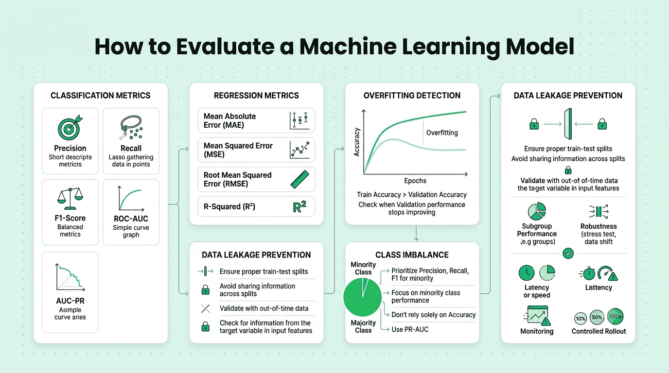
Answer: Precision measures the proportion of positive predictions that are actually correct (minimizing false positives); recall measures the proportion of actual positives the model correctly identifies (minimizing false negatives). Prioritization depends on the relative cost of each error type — high-stakes situations where missing a positive is costly favor recall, while situations where false positives are costly favor precision.
Explanation: One of the most fundamental and frequently tested model evaluation concepts, since choosing the wrong metric to optimize can produce a model that's technically accurate but practically useless.
Real-World Example: A cancer screening model should prioritize recall (minimizing missed diagnoses, even at the cost of more false alarms), while a spam filter should prioritize precision (minimizing legitimate emails incorrectly flagged as spam).
Common Mistakes: Optimizing for overall accuracy without considering the specific, differing costs of false positives versus false negatives for the actual business problem.
Follow-up Questions: What is the F1 score, and when would you use it instead of examining precision and recall separately? How would you choose a classification threshold to balance precision and recall for a specific use case? What is a precision-recall curve, and what does it show?
Question 12
Question: Explain the ROC curve and AUC, and their limitations.
Answer: A ROC curve plots true positive rate against false positive rate across all classification thresholds; AUC summarizes this into a single number representing the model's ability to rank positive examples higher than negative ones. A key limitation: AUC can be misleadingly optimistic on highly imbalanced datasets, since it's insensitive to actual class distribution — in those cases, a precision-recall curve/AUC-PR is often more informative.
Explanation: A very commonly used classification evaluation metric, with interviewers often specifically probing for awareness of its imbalanced-data limitation.
Real-World Example: A fraud detection model with 0.5% fraud prevalence might show a deceptively high AUC-ROC while still performing poorly on the metric that actually matters (precision at a usable recall level) — AUC-PR would more clearly reveal this weaker real-world performance.
Common Mistakes: Reporting AUC-ROC as the sole evaluation metric for a highly imbalanced problem without considering the more informative AUC-PR.
Follow-up Questions: Why is AUC-PR often more informative than AUC-ROC for imbalanced datasets? What does an AUC of 0.5 mean, and what would an AUC below 0.5 imply? How would you explain AUC to a non-technical stakeholder?
Question 13
Question: How would you evaluate a regression model, and what are the tradeoffs between common metrics?
Answer: MAE (mean absolute error) measures average absolute error, robust to outliers. MSE (mean squared error) penalizes larger errors disproportionately, sensitive to outliers. RMSE returns MSE to the original units for interpretability. R-squared measures the proportion of variance explained, useful for relative fit but potentially misleading without also examining absolute error magnitude.
Explanation: A foundational regression evaluation question, testing whether a candidate matches the right metric to the specific business tolerance for large versus small errors.
Real-World Example: A demand forecasting model where a large single-day miss is especially costly (causing stockouts) might prioritize minimizing RMSE, while a model where consistent moderate accuracy matters more might prioritize MAE.
Common Mistakes: Reporting only R-squared without also examining absolute error metrics in business-meaningful units.
Follow-up Questions: When would you prefer MAE over RMSE, and vice versa? What's a limitation of R-squared as a standalone metric, especially comparing models with different numbers of features? How would you communicate a regression model's expected error to a non-technical stakeholder?
Question 14
Question: How would you detect and address overfitting in a machine learning model?
Answer: Detection: compare training versus validation performance — a large gap indicates overfitting; a learning curve showing validation error diverging from training error as training progresses is another clear signal. Addressing it: gather more training data, simplify the model, apply regularization, use cross-validation for more reliable model selection, or apply early stopping for iterative models.
Explanation: One of the most fundamental practical machine learning skills, testing both diagnostic ability and a concrete remediation toolkit.
Real-World Example: A deep decision tree achieving 99% training accuracy but only 70% validation accuracy is a clear overfitting signal, addressable by limiting tree depth or switching to a regularized ensemble method.
Common Mistakes: Only looking at training performance, never comparing against a held-out validation/test set, missing overfitting entirely until poor production performance reveals it.
Follow-up Questions: How would you distinguish overfitting from a genuinely difficult, high-noise problem where even a well-fit model has limited accuracy? What's the difference between early stopping and regularization as remedies? How would you use a learning curve to diagnose whether more training data would actually help?
Question 15
Question: What is data leakage, and how would you detect and prevent it?
Answer: Data leakage occurs when information from outside the legitimate training dataset (often unavailable at real prediction time) influences model training, causing artificially inflated validation performance that fails to hold up in deployment. Prevention: carefully audit features for future or target-derived information, fit preprocessing steps only on training data, and use time-aware splitting for temporal data.
Explanation: One of the most consequential and commonly tested practical pitfalls, since leakage often produces a model that looks excellent in validation but fails or underperforms in production.
Real-World Example: A hospital readmission model accidentally including a "discharge disposition" feature (only known after the outcome being predicted has occurred) would show unrealistically strong validation performance that collapses once deployed.
Common Mistakes: Not carefully considering whether each feature would actually be available at the real moment of prediction, discovering leakage only after a suspiciously high-performing model fails to replicate its performance in production.
Follow-up Questions: Can you give another concrete example of data leakage? How would you specifically audit a feature engineering pipeline for it? What's target leakage, and how does it differ from train/test contamination?
Question 16
Question: How would you handle a machine learning problem with severe class imbalance?
Answer: Approaches include resampling (oversampling the minority class via SMOTE, or undersampling the majority class), adjusting class weights in the loss function, choosing appropriate evaluation metrics (precision, recall, F1, AUC-PR rather than raw accuracy), and considering an anomaly-detection framing if the imbalance is extreme.
Explanation: An extremely common and practically important real-world scenario, testing awareness of both technique options and why standard accuracy is misleading in this context.
Real-World Example: A fraud detection model trained on data where 0.1% of transactions are fraudulent would achieve 99.9% accuracy by trivially predicting "not fraud" for everything — requiring class weighting, resampling, and appropriate metrics to build a genuinely useful model.
Common Mistakes: Relying on raw accuracy as the primary metric for a severely imbalanced problem, which can be highly misleading and mask a model that's essentially useless for the minority class.
Follow-up Questions: What's the difference between SMOTE and simple random oversampling? How would you choose an appropriate classification threshold for an imbalanced problem, rather than the default 0.5? How would you communicate the precision/recall tradeoff to a business stakeholder for this kind of problem?
Question 17
Question: What is the difference between validation set performance and test set performance, and why do you need both?
Answer: A validation set is used during model development for hyperparameter tuning and model selection — since you're repeatedly evaluating on it, performance on the validation set can become optimistically biased through this iterative selection process. A held-out test set, used only once at the very end, provides an unbiased estimate of how the final chosen model will actually perform on genuinely unseen data.
Explanation: A foundational validation methodology concept, testing whether a candidate understands why a single train/test split isn't sufficient once any iterative model selection is involved.
Real-World Example: A team trying dozens of different model configurations and selecting the best one based on validation performance would get an overly optimistic sense of that model's true performance if they reported the validation score as the final result, rather than evaluating the finally-selected model once on a genuinely untouched test set.
Common Mistakes: Using the same held-out set for both iterative hyperparameter tuning and final performance reporting, effectively contaminating the "unbiased" estimate through repeated, implicit optimization against it.
Follow-up Questions: How would you handle this three-way split (train/validation/test) within a cross-validation scheme? What's nested cross-validation, and when would you use it? How would you communicate to a stakeholder why your reported test performance might differ from validation performance during development?
Question 18
Question: How would you evaluate whether a machine learning model is ready for production deployment?
Answer: Beyond standard offline metrics, consider: performance stability across relevant subgroups (not just in aggregate), robustness to realistic data quality issues and edge cases, latency/computational cost requirements for the production serving environment, a clear plan for ongoing monitoring, and, ideally, a controlled rollout (shadow deployment or small-scale A/B test) to validate real-world performance before a full launch.
Explanation: A holistic, practically-oriented question testing whether a candidate thinks beyond a single offline metric toward the full lifecycle of responsibly deploying a model.
Real-World Example: A model with strong aggregate accuracy might still perform poorly for a specific important subgroup — a shadow deployment comparing the new model's live predictions against the current production system's, without yet acting on them, can catch this before a risky full launch.
Common Mistakes: Treating a strong offline validation metric as sufficient justification for deployment without considering subgroup performance, latency constraints, or a post-launch monitoring plan.
Follow-up Questions: How would you design a shadow deployment or canary rollout for a new model? What ongoing monitoring would you put in place after deployment? How would you decide whether a model's performance on a specific important subgroup is acceptable, even if aggregate performance looks strong?
Part 3: Feature Engineering & Data Preprocessing
Question 19
Question: How would you handle missing data before training a machine learning model?
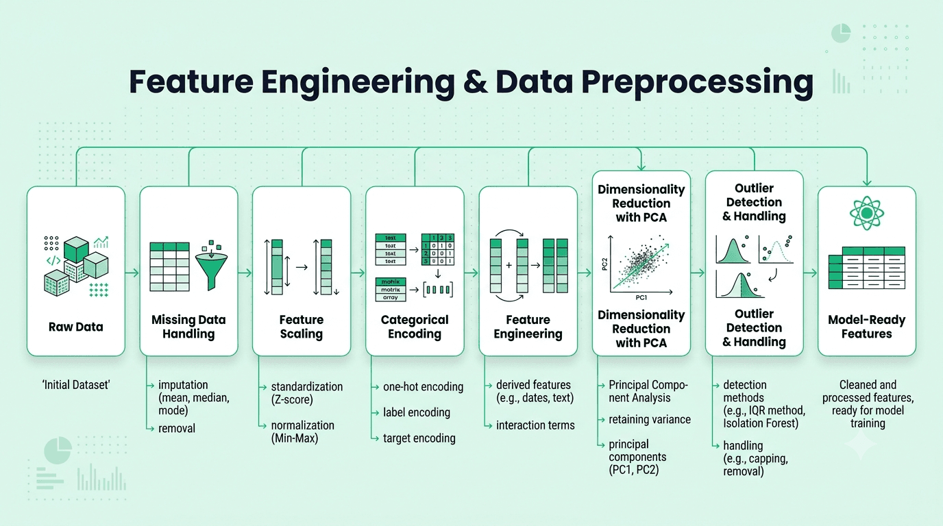
Answer: Options depend on the missingness mechanism and extent: drop rows/columns if missingness is minimal and random, impute with a statistic (mean/median/mode) or a more sophisticated model-based approach for moderate missingness, or create a separate "missing" indicator feature if the fact that a value is missing might itself carry predictive signal — critically, fit any imputation strategy only on training data to avoid leakage.
Explanation: A very commonly tested practical preprocessing question, since virtually every real-world dataset has missing values requiring a deliberate, justified handling strategy.
Real-World Example: In a customer dataset, a missing "income" value might be imputed with a segment-specific median while also adding a binary "income_was_missing" feature, since the fact of missingness might itself be predictive of certain behaviors.
Common Mistakes: Applying a single blanket imputation strategy without considering whether missingness might vary meaningfully by subgroup, or whether missingness itself carries useful signal.
Follow-up Questions: How would you decide between simple imputation and a more sophisticated model-based approach? How does the missing data mechanism (missing at random versus not at random) affect your chosen strategy? How would you handle missing data differently for a tree-based model versus a linear model?
Question 20
Question: What is feature scaling, and when is it necessary?
Answer: Feature scaling transforms features to a common scale, necessary for algorithms sensitive to feature magnitude and distance calculations (k-NN, SVM, gradient descent-based methods including neural networks and linear/logistic regression), but generally unnecessary for tree-based models, which split based on feature order/thresholds rather than magnitude.
Explanation: A very commonly tested practical concept, since applying (or failing to apply) scaling appropriately is a frequent source of both errors and unnecessary extra work.
Real-World Example: A k-NN model using both "age" (range roughly 0-100) and "income" (range potentially 0-500,000) without scaling would have distance calculations almost entirely dominated by the income feature simply due to its much larger raw numeric range.
Common Mistakes: Applying scaling unnecessarily to tree-based models, or forgetting it for models that genuinely require it.
Follow-up Questions: What's the difference between standardization and min-max normalization, and when would you choose one over the other? How would you correctly apply scaling within a cross-validation pipeline to avoid data leakage? Does scaling affect model interpretability or just optimization/performance?
Question 21
Question: How would you encode categorical variables for a machine learning model?
Answer: Common approaches: one-hot encoding (for nominal categories with reasonable cardinality), label/ordinal encoding (only appropriate when categories have genuine inherent order), and target/mean encoding (powerful for high-cardinality features, but requires careful cross-validation to avoid leakage).
Explanation: A very commonly tested practical preprocessing skill, testing whether a candidate matches the encoding method to the categorical variable's specific characteristics.
Real-World Example: A "zip code" feature with thousands of unique values would create an unwieldy dimensionality with one-hot encoding, making target encoding (with proper cross-validation) a more practical choice.
Common Mistakes: Using label/ordinal encoding for a nominal variable, which incorrectly implies a false numeric ordering the model may inadvertently learn from.
Follow-up Questions: What's the risk of target encoding causing data leakage, and how would you mitigate it? How would you handle a categorical feature with a category present in test data but not training data? How does encoding choice differ for tree-based versus linear models?
Question 22
Question: What is feature engineering, and why is it often more impactful than the choice of algorithm?
Answer: Feature engineering uses domain knowledge to create new input features from raw data that better expose the underlying patterns relevant to the prediction task — often having a larger impact than algorithm choice because even a sophisticated model can't learn a relationship if the necessary signal isn't present in some usable form within the input features at all.
Explanation: A very commonly tested, open-ended question assessing creativity and domain-application skill beyond purely technical/algorithmic knowledge.
Real-World Example: For a churn prediction model, engineering a "days since last login" and "trend in login frequency" feature often captures much more predictive signal than the raw timestamp alone, regardless of which algorithm is ultimately used.
Common Mistakes: Relying entirely on raw features "as-is" without applying domain knowledge to construct more informative derived features.
Follow-up Questions: Can you walk through your feature engineering process for a project you've worked on? How would you avoid creating a feature that inadvertently causes data leakage? How would you evaluate whether a newly engineered feature is actually adding value?
Question 23
Question: What is Principal Component Analysis (PCA), and when would you use it?
Answer: PCA is a dimensionality reduction technique that transforms correlated features into a smaller set of uncorrelated components, ordered by the amount of variance they capture, allowing you to retain most of the informative variance while discarding lower-variance, often noisier dimensions.
Explanation: A very commonly used and tested technique for high-dimensional data, both to reduce computational cost and overfitting risk.
Real-World Example: A dataset with hundreds of highly correlated financial indicators might be reduced to a handful of principal components capturing most of the original variance, simplifying downstream modeling and reducing overfitting risk.
Common Mistakes: Not standardizing features before PCA (since it's sensitive to feature scale), or treating resulting components as retaining the original features' direct interpretability.
Follow-up Questions: How would you decide how many principal components to retain? How does PCA differ from t-SNE/UMAP for dimensionality reduction, especially for visualization? What's the limitation of PCA for capturing non-linear relationships in data?
Question 24
Question: How would you detect and handle outliers before or during model training?
Answer: Detection methods include visual inspection (box plots), statistical thresholds (values beyond 1.5×IQR, or several standard deviations), and model-based approaches (isolation forests). Handling depends on the cause: correct data entry errors, consider removing or capping (winsorizing) genuine extreme values that would unduly distort training, or use robust techniques less sensitive to outliers if they're legitimate and shouldn't be discarded.
Explanation: A practical data preprocessing skill, testing thoughtful judgment rather than a reflexive "always remove outliers" approach.
Real-World Example: In a dataset of customer order values, a $1 million order might be a legitimate large B2B transaction (should likely be retained) or a data entry error (should be corrected) — appropriate handling depends entirely on investigation.
Common Mistakes: Automatically removing all statistical outliers without investigating whether they represent genuine, important data points.
Follow-up Questions: How would outlier handling differ for linear regression versus a tree-based model? What is winsorizing, and how does it differ from removing outliers? How would you detect multivariate outliers that might not appear extreme on any single feature individually?
FREE TO USE
8k+ SESSIONS92% FLUENCY4.9★ RATING
Speak With Confidence
Real Conversations. Real Scenarios. Speak until it feels natural.
- Real-Time Speaking Practice
- Guided Conversation Flows
- Instant AI Feedback
Part 4: Deep Learning & Neural Networks
Question 25
Question: Explain how backpropagation works in training a neural network.
Answer: Backpropagation computes the gradient of the loss function with respect to each weight by applying the chain rule of calculus, propagating error backward from the output layer through each hidden layer to the input layer — these gradients are then used by an optimizer (like gradient descent) to update each weight in the direction that reduces loss.
Explanation: The foundational algorithm underlying how virtually all neural networks are trained, a very commonly tested concept to gauge whether a candidate understands the mechanics beneath the "black box" of deep learning frameworks.
Real-World Example: Every call to .backward() in PyTorch or TensorFlow during training performs automatic differentiation implementing backpropagation, whether for an image classifier or a large language model.
Common Mistakes: Describing backpropagation only vaguely ("it adjusts weights based on error") without connecting it to the chain rule propagating gradients layer by layer backward.
Follow-up Questions: What is the vanishing gradient problem, and how does it relate to backpropagation in deep networks? What role does the learning rate play in how gradients update weights? How does backpropagation differ for a recurrent neural network (backpropagation through time)?
Question 26
Question: What is the vanishing/exploding gradient problem, and how is it addressed in modern deep learning?
Answer: In deep networks, gradients can become extremely small (vanishing) or extremely large (exploding) as they propagate backward through many layers, especially with certain activation functions — making very deep networks difficult to train. Solutions include ReLU-family activation functions, careful weight initialization, batch normalization, gradient clipping, and architectural innovations like residual/skip connections.
Explanation: A foundational deep learning challenge, and understanding it motivates many standard architectural and training choices used in modern networks.
Real-World Example: Training very deep convolutional networks became practical largely due to residual connections (ResNet), which provide a more direct path for gradients to flow backward, substantially mitigating vanishing gradients that had previously limited network depth.
Common Mistakes: Not connecting the problem to specific, concrete solutions (ReLU, batch norm, residual connections), giving only an abstract description.
Follow-up Questions: Why does ReLU help mitigate vanishing gradients compared to sigmoid? What is gradient clipping, and how does it specifically address exploding gradients? How do residual connections help gradients flow through very deep networks?
Question 27
Question: What is dropout, and how does it help prevent overfitting in neural networks?
Answer: Dropout randomly deactivates a proportion of neurons during each training iteration, forcing the network to not over-rely on any single neuron or co-adapted group, effectively training an implicit ensemble of "thinned" sub-networks combined approximately at inference time when dropout is turned off.
Explanation: A very commonly used and tested regularization technique specific to neural networks.
Real-World Example: A large network trained on a relatively modest amount of labeled data would likely overfit without regularization; applying dropout (commonly 0.2-0.5 in fully connected layers) is a standard, effective technique to substantially reduce this risk.
Common Mistakes: Forgetting dropout should be disabled at inference/test time, and not being able to explain the "implicit ensemble" intuition behind why it works.
Follow-up Questions: How does dropout's behavior differ between training and inference? How would you choose an appropriate dropout rate for a specific layer? How does dropout relate to and differ from L2 weight decay?
Question 28
Question: What is the Transformer architecture, and what role does self-attention play?
Answer: The Transformer processes an entire sequence in parallel using a self-attention mechanism that allows each position to directly weigh and incorporate information from every other position, dynamically learning relevance — enabling much better parallelization during training than RNNs and more effective modeling of long-range dependencies.
Explanation: A very current and increasingly essential architecture to understand, given its role underlying nearly all modern large language models.
Real-World Example: Modern LLMs are built on the Transformer architecture, whose self-attention mechanism allows a model to correctly resolve which earlier noun a pronoun refers to in a long, complex sentence, a task difficult for purely sequential architectures.
Common Mistakes: Naming "attention" without explaining the core intuition (each token dynamically attending to relevant other tokens) or why it enables better parallelization than RNNs.
Follow-up Questions: What is multi-head attention, and why use multiple heads? How does positional encoding address self-attention's lack of inherent sequence order awareness? What's the difference between encoder-only, decoder-only, and encoder-decoder Transformer architectures?
Question 29
Question: What is batch normalization, and why is it commonly used in deep networks?
Answer: Batch normalization normalizes the inputs to each layer using the mean and variance computed across the current mini-batch during training, stabilizing and accelerating training by reducing internal covariate shift, allowing higher learning rates, and providing a mild regularization effect.
Explanation: A widely used and commonly tested deep learning technique, testing both mechanism and practical training benefits.
Real-World Example: Very deep convolutional networks commonly include batch normalization after convolutional layers specifically because it dramatically speeds up and stabilizes training convergence compared to networks without it.
Common Mistakes: Not knowing how batch normalization behaves differently at inference time (using running statistics rather than current batch statistics).
Follow-up Questions: How does batch normalization's behavior differ between training and inference? What's the difference between batch normalization and layer normalization, and when would you prefer each (e.g., in Transformers)? How does batch size affect batch normalization's stability?
Question 30
Question: How would you decide whether a problem calls for deep learning versus a simpler traditional ML model?
Answer: Consider data type and volume (deep learning generally excels with large amounts of unstructured data like images or text, while traditional ML like gradient boosting often matches or exceeds it on smaller, structured/tabular datasets), the complexity of the underlying patterns, and practical constraints like interpretability, compute, latency, and team expertise.
Explanation: A very important, frequently tested judgment question, since deep learning isn't universally superior and the choice should be driven by problem characteristics.
Real-World Example: A tabular customer churn prediction problem with a moderate number of engineered features often performs just as well (or better, with more interpretability and less compute) using gradient boosting rather than a deep neural network.
Common Mistakes: Defaulting to deep learning purely because it's fashionable, without considering whether the problem's data type and volume actually justify the added complexity.
Follow-up Questions: Can you give an example from your own experience where you chose a simpler model over deep learning, and why? What are the key practical tradeoffs between deep learning and traditional ML approaches? How does dataset size specifically affect this decision?
Question 31
Question: What is transfer learning, and when is it useful?
Answer: Transfer learning takes a model pretrained on a large, related dataset/task and adapts (fine-tunes) it for a new, often smaller, related task, leveraging previously learned general representations rather than training from scratch — particularly valuable when labeled data for the new task is limited.
Explanation: An increasingly important concept, especially in deep learning, testing awareness of a technique that dramatically reduces data and compute requirements for many real applications.
Real-World Example: A company building an image classifier with only a few thousand labeled images would typically fine-tune a large model pretrained on millions of general images, dramatically improving performance given the limited task-specific data.
Common Mistakes: Attempting to train a large, complex model entirely from scratch on a small dataset when a pretrained, fine-tuned model would likely perform significantly better with far less data.
Follow-up Questions: How would you decide how many layers to freeze versus fine-tune? What's the difference between feature extraction and fine-tuning as transfer learning strategies? What risks arise if the pretrained model's original data is very different from your new task's domain?
Question 32
Question: What is an embedding, and why are embeddings useful in machine learning?
Answer: An embedding is a learned, dense, lower-dimensional vector representation of a discrete or high-dimensional input, positioned in a continuous vector space such that semantically or functionally similar items end up close together — capturing rich, useful relationships that a simple one-hot encoding cannot represent.
Explanation: A foundational and increasingly important concept given the prominence of embedding-based techniques across recommendation systems, NLP, and search/retrieval applications.
Real-World Example: Word embeddings position semantically similar words close together in vector space, enabling models to generalize based on meaning rather than treating each word as an independent, unrelated category.
Common Mistakes: Confusing embeddings with simple dimensionality reduction like PCA, without recognizing embeddings are typically learned to optimize a specific downstream task or self-supervised objective.
Follow-up Questions: How would you evaluate the quality of a set of learned embeddings? What's the difference between a pretrained embedding and one learned end-to-end for a specific task? How are embeddings used in a modern retrieval-augmented generation system?
Part 5: ML Systems, Deployment & MLOps
Question 33
Question: What is model drift, and how would you detect and address it in a production model?
Answer: Model drift occurs when a deployed model's performance degrades over time because the statistical properties of incoming data (data/covariate drift) or the relationship between features and target (concept drift) change from what the model was trained on. Detection involves ongoing performance monitoring against ground truth when available, and statistical comparison of live feature distributions against training data. Addressing it typically involves scheduled or trigger-based retraining.
Explanation: A critical, very commonly tested production ML concept, since a model's real-world value depends on maintaining performance after deployment, not just at launch.
Real-World Example: A demand forecasting model trained on pre-pandemic consumer behavior experienced significant concept drift when the pandemic dramatically shifted purchasing patterns, requiring urgent retraining on more recent data.
Common Mistakes: Deploying a model without any ongoing monitoring plan, assuming initial strong validation performance will persist indefinitely.
Follow-up Questions: What's the difference between data drift and concept drift, and can you give an example of each? How would you decide on an appropriate retraining cadence? What would you do if ground-truth labels for calculating live performance are only available with significant delay?
Question 34
Question: What is the difference between batch and real-time (online) model inference?
Answer: Batch inference generates predictions for a large set of inputs on a scheduled basis, storing results for later use, appropriate when predictions can tolerate some staleness. Real-time inference generates predictions on-demand in response to individual requests, typically with strict low-latency requirements, necessary when predictions must reflect the most current available information.
Explanation: A foundational production ML architecture decision, testing practical judgment about matching the serving approach to actual latency and freshness requirements.
Real-World Example: A weekly email marketing recommendation model can comfortably use batch inference, while a real-time fraud detection system checking each transaction requires online inference with sub-second latency.
Common Mistakes: Defaulting to complex real-time infrastructure for a use case that doesn't actually require it, unnecessarily increasing system complexity and cost.
Follow-up Questions: What infrastructure considerations differ between building a batch versus real-time inference pipeline? How would you handle a situation where required features for real-time inference aren't available with low enough latency? What is a feature store, and how does it help bridge batch and real-time feature consistency?
Question 35
Question: What is a feature store, and what problem does it solve?
Answer: A feature store centralizes storage, management, and serving of machine learning features consistently across both training and real-time inference, solving the common and consequential problem of "training-serving skew" — where features computed differently between the training and serving pipelines cause a model to behave unexpectedly or perform worse than expected in production.
Explanation: An increasingly important and commonly tested MLOps concept, especially at organizations building and deploying many models.
Real-World Example: A feature computed as "average purchase amount over the last 30 days" might be calculated slightly differently offline versus in a real-time serving pipeline (different rounding, time zone handling) — a feature store helps ensure both compute it identically.
Common Mistakes: Maintaining entirely separate, independently-implemented feature computation logic for training versus serving without any shared source of truth.
Follow-up Questions: How does a feature store typically handle both batch and real-time feature computation needs? How would you detect training-serving skew if you didn't have a feature store? What are some well-known feature store platforms you're aware of?
Question 36
Question: How would you design an A/B test to validate a new machine learning model before a full production rollout?
Answer: Consider a shadow deployment first (running the new model alongside production on live traffic without acting on its predictions), followed by a proper randomized A/B test allocating a portion of live traffic to the new model and measuring the actual downstream business metric impact, not just an offline validation metric, before full rollout.
Explanation: Tests the ability to connect model evaluation methodology with broader experimentation and safe deployment practices.
Real-World Example: Before fully replacing a production recommendation model, a company might first run it in shadow mode to confirm stability, then run an A/B test to confirm it actually improves the real business metric (like revenue), not just an offline proxy metric.
Common Mistakes: Relying solely on strong offline validation metrics to justify full production rollout without any live testing.
Follow-up Questions: How would you decide on an appropriate percentage of traffic for the A/B test phase? What would you do if the new model shows strong offline improvement but no significant live business metric improvement? How would you design a safe, gradual rollout plan with an appropriate rollback trigger?
Question 37
Question: What is model interpretability, and what techniques would you use to explain a complex model's predictions?
Answer: Model interpretability is the ability to understand and explain why a model produced a specific prediction, important for trust, debugging, and fairness auditing. Techniques include SHAP (consistent feature attribution based on game theory), LIME (approximating a model's local behavior with a simpler, interpretable model), and partial dependence plots (showing a feature's average marginal effect).
Explanation: An increasingly important and commonly tested topic given growing regulatory and business demand for explainable AI, especially in high-stakes domains.
Real-World Example: A bank using a complex gradient boosting model for loan approval might use SHAP values to explain to a rejected applicant which factors most contributed to their application's rejection.
Common Mistakes: Treating SHAP or LIME as providing a definitive causal explanation of the model's true internal reasoning rather than an approximation of feature attribution.
Follow-up Questions: How does SHAP differ from LIME in its underlying approach and guarantees? How would you use these techniques to investigate potential model bias against a protected group? What are the tradeoffs between an inherently interpretable model and a complex model with post-hoc explanation?
Question 38
Question: How would you approach a situation where a model performs well offline but poorly once deployed to production?
Answer: Systematic investigation: check for training-serving skew (are features computed identically in both pipelines?), verify production data actually matches the training/validation distribution, review the offline evaluation methodology for potential data leakage, and examine whether the offline metric genuinely aligns with the real business metric being measured in production.
Explanation: A very practical, frequently tested troubleshooting scenario, since this specific gap between offline and online performance is one of the most common real-world production ML problems.
Real-World Example: A model showing excellent offline accuracy but poor live performance might be traced to a subtle bug where a feature was computed using future information during offline evaluation (data leakage) unavailable at real-time prediction.
Common Mistakes: Assuming production infrastructure must be broken as the first hypothesis, without first re-examining the offline evaluation methodology for leakage or a mismatched metric choice.
Follow-up Questions: How would you systematically rule out data leakage as the cause of an offline-online performance gap? How would you specifically check for training-serving feature skew? What would you do if you confirmed production data has genuinely, legitimately drifted from training data?
Question 39
Question: How would you set up monitoring for a machine learning model in production?
Answer: Monitor multiple layers: system/operational health (latency, error rates), input data quality and distribution (checking for drift), prediction distribution (unexpected shifts over time), and actual model performance against ground truth once available — combined with alerting thresholds and clear escalation when anomalies are detected.
Explanation: A foundational MLOps question testing holistic understanding of what needs to be tracked beyond just the initial offline validation metric.
Real-World Example: A credit risk model might have automated alerts if the proportion of applications flagged as high-risk suddenly spikes well beyond historical norms, prompting investigation before delayed ground-truth default outcomes directly confirm a performance problem.
Common Mistakes: Only monitoring system-level operational metrics without any monitoring of data quality or prediction distribution, missing early warning signs of degrading model performance.
Follow-up Questions: How would you set appropriate alerting thresholds balancing catching real issues against false alarms? How would you monitor performance when ground truth labels are delayed by weeks or months? What would you do if you detected a sudden, significant shift in input feature distribution?
Question 40
Question: How would you approach versioning and reproducibility for a machine learning project?
Answer: Version control the code, track and version the specific dataset(s) used for training, log experiment configurations, hyperparameters, and metrics for every training run (using an experiment tracking tool), and version/register trained model artifacts with clear metadata linking each model back to the exact code, data, and configuration that produced it.
Explanation: A foundational MLOps practice, increasingly expected of ML practitioners given the growing maturity of production ML engineering standards.
Real-World Example: When a production model's performance unexpectedly changes, comprehensive experiment tracking and data versioning allows a team to quickly compare the current model against previous versions and pinpoint exactly what changed.
Common Mistakes: Tracking only code in version control while treating datasets, hyperparameters, and experiment results as an afterthought.
Follow-up Questions: What experiment tracking tools have you used, and what was your experience? How would you version a large dataset that changes frequently without duplicating it in full each time? How would you ensure reproducibility with inherently stochastic training processes like random weight initialization?
Part 6: Scenario-Based, Case Studies & Industry Trends
Question 41
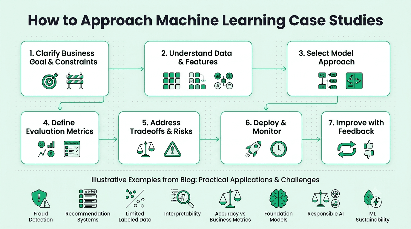
Question: How would you approach designing a machine learning system to detect fraudulent transactions?
Answer: Clarify business context and constraints (acceptable latency, cost of false positives versus false negatives), propose relevant features (transaction attributes, historical behavior, device/location signals), select an appropriate model family (often gradient boosting for structured fraud data), define evaluation metrics appropriate for the imbalanced, cost-sensitive nature of fraud, and address deployment considerations (real-time latency, a feedback loop for continuously incorporating newly confirmed labels).
Explanation: One of the most commonly asked open-ended system design case studies, testing end-to-end thinking across the entire ML problem lifecycle.
Real-World Example: Real production fraud detection systems typically combine a real-time ML model with rule-based guardrails and a human review queue for borderline cases, reflecting the genuinely high stakes and cost asymmetry involved.
Common Mistakes: Jumping immediately into model architecture details without first clarifying business constraints and cost tradeoffs that should drive those downstream technical decisions.
Follow-up Questions: How would you handle the severe class imbalance inherent to fraud detection? How would you design a feedback loop to continuously improve the model with newly confirmed labels? How would you balance real-time latency requirements against a more complex, higher-accuracy model?
Question 42
Question: How would you approach designing a recommendation system for an e-commerce platform?
Answer: Clarify the specific business goal, consider cold-start challenges for new users or products, evaluate collaborative filtering versus content-based approaches versus a hybrid, and define both offline evaluation metrics (like precision@k) and, critically, a plan for online A/B testing, since offline recommendation metrics don't always translate directly to real user behavior improvement.
Explanation: Another very commonly asked open-ended system design case study, testing structured problem decomposition for a canonical business ML application.
Real-World Example: Major e-commerce platforms typically combine collaborative filtering for established users/products with content-based approaches specifically for cold-start scenarios, often further blended with business-rule-based boosting for strategic priorities.
Common Mistakes: Not addressing the cold-start problem, or relying solely on offline evaluation metrics as sufficient proof of real-world business value.
Follow-up Questions: How would you specifically address the cold-start problem for new users or new products? How would you balance recommendation relevance against beneficial diversity in the results shown? How would you evaluate whether the system is creating an unhealthy filter bubble over time?
Question 43
Question: How would you decide between a simpler, more interpretable model and a more complex, higher-performing "black box" model for a given project?
Answer: Weigh the specific business context's requirements — regulatory/compliance needs for explainability, the stakes and reversibility of decisions the model informs, the actual magnitude of the performance difference between options, and the team's ongoing ability to maintain and debug the chosen approach — rather than defaulting to either extreme.
Explanation: A common behavioral/scenario question testing practical judgment about a very real and frequent tradeoff in applied ML work.
Real-World Example: A candidate might describe choosing a more interpretable logistic regression over a marginally higher-performing neural network for a credit decisioning use case specifically because of regulatory requirements mandating clear, auditable explanations for adverse decisions.
Common Mistakes: Describing a decision made purely based on personal technical preference without connecting the choice to the specific, concrete business context that should genuinely drive this tradeoff.
Follow-up Questions: How did you quantify or communicate the performance difference between the two options to stakeholders? What would have changed your decision toward the more complex model? How do you generally approach explaining this tradeoff to stakeholders who might not initially understand why you wouldn't simply choose the "best" performing model?
Question 44
Question: A stakeholder tells you your model's accuracy needs to be "as high as possible." How would you respond and reframe the conversation?
Answer: Explain that model accuracy is only one dimension, and that "as high as possible" without a defined threshold or business context isn't actionable — probe for the actual decision the model informs and the relative cost of false positives versus false negatives for that specific use case, since the right metric and appropriate performance target depend entirely on that context, not a universal maximum.
Explanation: A commonly tested scenario testing the ability to translate a vague, non-technical request into a well-defined, technically tractable problem.
Real-World Example: A "high accuracy" request for a fraud model without any further context might actually need to prioritize recall over raw accuracy, given the severe class imbalance and the very different real costs of a missed fraud case versus a false alarm.
Common Mistakes: Simply pursuing the highest raw accuracy number possible without pushing back to clarify what business outcome and cost tradeoff should actually be driving the metric choice.
Follow-up Questions: How would you determine the appropriate target metric and threshold together with this stakeholder? How would you communicate the precision/recall tradeoff in terms the stakeholder would find genuinely meaningful? What would you do if the stakeholder insists on "accuracy" despite your explanation of why it's the wrong metric here?
Question 45
Question: How would you approach a project where the available labeled training data is very limited?
Answer: Consider transfer learning from a pretrained model to reduce the amount of task-specific labeled data needed, active learning to prioritize labeling the most informative examples, data augmentation to synthetically expand the effective training set, semi-supervised techniques leveraging unlabeled data, or, if feasible, investing in additional targeted data collection/labeling before committing to full-scale model development.
Explanation: A commonly tested, practical scenario testing resourcefulness for a genuinely common real-world constraint.
Real-World Example: A team with only a few hundred labeled images for a specialized defect-detection task would typically fine-tune a large pretrained image model rather than training a new model from scratch, dramatically improving performance given the limited labeled data available.
Common Mistakes: Attempting to train a complex model from scratch on a genuinely insufficient amount of labeled data, producing an unreliable model rather than using techniques specifically suited to limited-data scenarios.
Follow-up Questions: How would you decide between active learning and simply collecting more random labeled data? What data augmentation techniques would be appropriate for your specific data type? How would you validate a model trained on such a limited dataset to have genuine confidence in its real-world performance?
Question 46
Question: How would you communicate a machine learning model's limitations and appropriate use boundaries to a non-technical stakeholder deploying it in a business process?
Answer: Explain performance in concrete, business-relevant terms (not raw statistical metrics), be explicit about the specific conditions under which the model is reliable versus where its confidence and accuracy genuinely degrade, and recommend appropriate human oversight or fallback processes for cases outside the model's validated scope, rather than presenting the model as universally reliable.
Explanation: A commonly tested communication and responsible-deployment question, testing whether a candidate proactively communicates limitations rather than only touting performance.
Real-World Example: A model trained primarily on data from one customer segment should be explicitly flagged as potentially less reliable for other segments it wasn't well-validated on, with an appropriate human review process recommended for those cases rather than blind trust in the model's output.
Common Mistakes: Presenting only aggregate performance metrics to a stakeholder without discussing where and how the model's reliability actually degrades, risking overconfident deployment in scenarios the model wasn't genuinely validated for.
Follow-up Questions: How would you identify the specific conditions under which your model's performance meaningfully degrades? How would you design a human-in-the-loop fallback process for low-confidence predictions? How would you monitor for cases in production that fall outside the model's validated scope?
Question 47
Question: How is the rise of foundation models and large pretrained models changing how machine learning practitioners approach new projects?
Answer: Many tasks previously requiring training a custom model from scratch can now be addressed by prompting or fine-tuning a large pretrained foundation model, significantly reducing the data and engineering investment needed for many applications — shifting practitioner focus toward effectively adapting, evaluating, and integrating these models rather than always building bespoke architectures, though traditional ML approaches (especially for structured/tabular data) often remain more effective and efficient for many use cases.
Explanation: A highly current and increasingly frequently tested trend question, testing whether a candidate has genuine, up-to-date perspective on how the field is evolving.
Real-World Example: A task like classifying customer support tickets by topic, which previously required building and labeling data for a custom text classification model, can often be accomplished quickly today using a well-prompted foundation model or one fine-tuned on a much smaller labeled dataset than would have been previously needed.
Common Mistakes: Assuming foundation models are now the best approach for every problem type, without recognizing that traditional ML methods often still substantially outperform them on structured/tabular data problems.
Follow-up Questions: How would you decide whether a foundation-model-based approach or a traditional custom-trained model is more appropriate for a specific task? What are the risks (cost, latency, hallucination) of using a large foundation model in a production ML pipeline? How do you think core ML practitioner skills will continue to shift as these models mature?
Question 48
Question: What is the growing importance of responsible AI and algorithmic fairness, and how would you evaluate a model for potential bias?
Answer: Responsible AI practices involve proactively assessing whether a model's predictions or errors disproportionately affect specific protected groups, using fairness metrics (like demographic parity or equalized odds, each capturing a different, sometimes mutually incompatible definition of fairness) to quantify disparities, and considering both technical mitigations and broader process changes like more diverse training data or human review for high-stakes decisions.
Explanation: An increasingly important and commonly tested topic given growing regulatory scrutiny and genuine ethical importance.
Real-World Example: A hiring screening model showing a significantly higher false-negative rate for a specific demographic group compared to others represents a fairness concern requiring investigation, regardless of the model's strong aggregate accuracy.
Common Mistakes: Assuming simply removing a protected attribute from model input is sufficient to ensure fairness, without recognizing correlated proxy features can still allow the model to indirectly learn similar biased patterns.
Follow-up Questions: Why can different fairness metrics be mathematically incompatible with each other, and how would you decide which is most appropriate for a given context? How would you investigate whether a model is exhibiting proxy discrimination through correlated features? What organizational processes would you recommend to catch fairness issues before production?
Question 49
Question: How is the growing focus on AI/ML sustainability and computational efficiency affecting model development practice?
Answer: Increasing awareness of the significant computational cost of training and serving large models is driving greater attention to efficiency: choosing appropriately-sized models rather than defaulting to the largest option, model distillation and quantization to reduce serving costs, and more careful cost-benefit evaluation of whether a marginal performance improvement from a much larger model genuinely justifies its increased resource cost.
Explanation: An increasingly relevant and commonly tested trend, testing awareness of practical efficiency considerations beyond pure predictive performance alone.
Real-World Example: A company deploying a customer-facing model might use a smaller, distilled or fine-tuned model for many routine queries rather than a massive general-purpose model, substantially reducing serving costs and latency while maintaining acceptable quality for that specific use case.
Common Mistakes: Defaulting to the largest, most powerful available model regardless of the task's actual complexity, without weighing real-world cost, latency, and environmental impact against the marginal performance benefit.
Follow-up Questions: What is model distillation, and how does it work at a high level? How would you decide whether a smaller, more efficient model is "good enough" for a specific production use case? How do you think about the tradeoff between model performance and computational cost in your own work?
Question 50
Question: How do you personally stay current with the rapidly evolving field of machine learning?
Answer: A strong answer describes a concrete, ongoing approach: following relevant research (papers, conference proceedings, well-curated technical blogs), participating in relevant technical communities, hands-on experimentation with new tools and techniques on personal or work projects, and periodically and critically reassessing whether a given newly emerging technique is genuinely worth adopting into regular practice versus representing short-lived hype.
Explanation: A very common closing question testing genuine intellectual curiosity and professional growth mindset, particularly important given how quickly the field continues to evolve.
Real-World Example: A candidate might describe regularly reading specific technical publications or following particular researchers, combined with periodically implementing and experimenting hands-on with a promising new technique or paper before considering recommending its adoption at work.
Common Mistakes: Giving a vague, generic answer without any specific, concrete examples of resources, communities, or particular recent techniques genuinely learned and evaluated.
Follow-up Questions: What's a specific recent development in the field you've found particularly interesting, and why? Can you name a few specific resources you follow regularly? How do you decide which emerging trends are genuinely worth investing meaningful time in versus likely transient hype?
How to Use This Guide
1. Don't memorize word-for-word. Use the "Explanation" sections to build genuine understanding, then practice explaining answers in your own words out loud.
2. Prioritize by role emphasis. Research-heavy or applied ML engineering roles should weight Parts 1 and 4 more heavily. Roles at companies with mature ML platforms should focus extra attention on Part 5. Product-facing roles should emphasize Part 6's case studies.
3. Practice the technical questions hands-on. Reading isn't enough for Parts 1-4 — actually implement and experiment with these concepts in code, including edge cases, ideally under mild time pressure to simulate a live technical screen.
4. Work through the case studies out loud. For Part 6's open-ended design questions, practice structuring your answer verbally (clarify requirements, propose an approach, discuss tradeoffs, address evaluation and deployment) since interviewers evaluate your structured thinking as much as your final answer.
5. Use follow-up questions as a self-check. After answering a question, try answering its follow-ups too — this is usually where interviews go deeper and where candidates get caught unprepared.
Good luck with your interview preparation.
More Blogs

Sep 28, 2026
Machine Learning Engineer Interview Preparation Guide: A Complete Roadmap for 2026
27 min read