Loading...
Contents
Top 100 Data Scientist Interview Questions
Aug 7, 2026149 min readUpdated Sep 18, 2026
A Comprehensive Preparation Guide
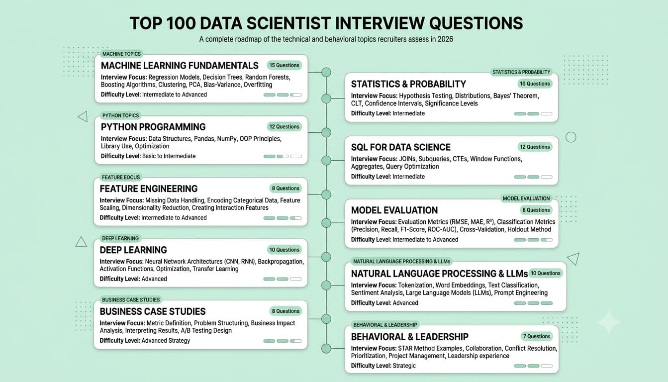
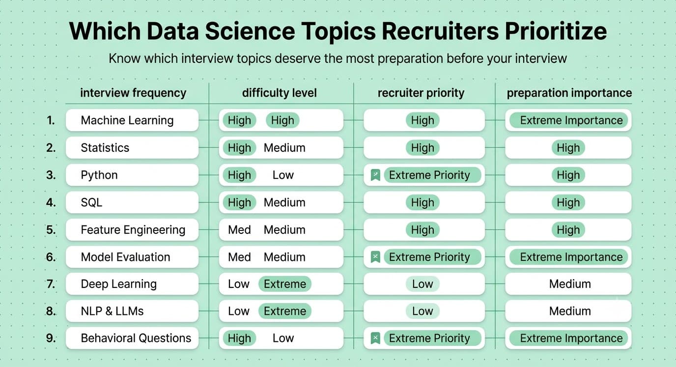
This guide covers the 100 most important data scientist interview questions, organized by topic and roughly ordered by frequency/importance within each category, progressing from statistical foundations through machine learning, deep learning, engineering practice, and business application.
Categories:
- Statistics & Probability Foundations (Q1-15)
- Machine Learning Fundamentals (Q16-30)
- Model Evaluation & Validation (Q31-40)
- Feature Engineering & Data Preprocessing (Q41-48)
- Deep Learning & Neural Networks (Q49-58)
- SQL & Python for Data Science (Q59-68)
- Experimentation & Causal Inference (Q69-76)
- MLOps & Model Deployment (Q77-84)
- Case Studies & Business/Stakeholder Scenarios (Q85-92)
- Industry Trends (Q93-100)
Read More : Data Science interview preparation guide 2026
FREE TO USE
25K+ INTERVIEWS4.8★ RATING68% IMPROVEMENT
Crack Your Dream Job
Real Interviews. Real Pressure. Practice until it feels easy.
- Seamless Interview Experience
- Resume & JD Questions
- Instant Personalized Feedback
Part 1: Statistics & Probability Foundations
Question 1
Question: What is the Central Limit Theorem, and why is it foundational to statistical inference?
Answer: The Central Limit Theorem (CLT) states that the sampling distribution of the sample mean approaches a normal distribution as sample size increases, regardless of the underlying population's distribution shape, provided the samples are independent and identically distributed with finite variance. This justifies using normal-distribution-based methods (confidence intervals, hypothesis tests) even when the underlying data itself isn't normally distributed.
Explanation: The CLT is the theoretical backbone that makes most classical inferential statistics valid in practice, since real-world data is rarely perfectly normal.
Real-World Example: Even if individual user session durations are heavily right-skewed, the average session duration computed from repeated large samples will be approximately normally distributed, justifying the use of t-tests to compare average session duration between two product variants.
Common Mistakes: Confusing the CLT (about the distribution of a sample statistic) with a claim that the underlying raw data becomes normal it does not; only the sampling distribution of the mean does, as sample size grows.
Follow-up Questions: How large does a sample need to be for the CLT to reasonably apply? How does the CLT relate to why we can use z-tests and t-tests? What happens to the standard error as sample size increases?
Question 2
Question: Explain the difference between Type I and Type II errors, and how they relate to statistical power.
Answer: A Type I error (false positive) occurs when you reject a true null hypothesis; its probability equals the significance level, alpha. A Type II error (false negative) occurs when you fail to reject a false null hypothesis; its probability is beta. Statistical power (1 - beta) is the probability of correctly detecting a true effect when one exists — increasing power (e.g., via larger sample size) generally reduces Type II error risk but doesn't directly change Type I error risk, which is set by your chosen alpha.
Explanation: Core hypothesis-testing vocabulary tested extensively because these tradeoffs directly inform real business/product decisions about acceptable risk.
Real-World Example: In a churn-prediction model deployed to trigger retention outreach, a Type I error means wasting outreach on a customer who wouldn't have churned, while a Type II error means missing a customer who does churn the acceptable balance depends on the relative cost of each error to the business.
Common Mistakes: Confusing which error is "false positive" versus "false negative," or not being able to connect the abstract concepts to a concrete cost-tradeoff scenario.
Follow-up Questions: How would you decide the appropriate significance threshold for a specific business context? What is a power analysis, and when would you conduct one before an experiment? How does increasing sample size affect Type I versus Type II error rates?
Question 3
Question: What is Bayes' Theorem, and how does Bayesian reasoning differ from frequentist statistics?
Answer: Bayes' Theorem describes how to update the probability of a hypothesis given new evidence: P(H|E) = P(E|H) × P(H) / P(E). Bayesian statistics treats probability as a degree of belief that gets updated with new data (starting from a prior belief and updating to a posterior), while frequentist statistics treats probability as the long-run frequency of events across repeated trials and doesn't incorporate prior beliefs formally into the analysis.
Explanation: A foundational conceptual question testing whether a candidate understands not just the formula but the philosophical distinction underlying two major statistical paradigms, both used in real data science work.
Real-World Example: A spam filter uses Bayes' Theorem directly (Naive Bayes classifier), updating the probability an email is spam based on the presence of specific words, starting from a prior probability (overall spam rate) and updating based on observed word evidence.
Common Mistakes: Being able to state the formula but not explain the practical difference in how Bayesian versus frequentist approaches would tackle the same real problem differently.
Follow-up Questions: Can you walk through a concrete Bayes' Theorem calculation (e.g., a medical testing false-positive example)? When would you prefer a Bayesian approach over a frequentist one in practice? What is a conjugate prior, and why is it computationally convenient?
Question 4
Question: What is the difference between correlation and causation, and what methods can help establish causation from observational data?
Answer: Correlation measures statistical association but doesn't imply one variable causes another a confounder, reverse causation, or coincidence could explain it. Establishing causation typically requires a randomized controlled experiment, or, when unavailable, quasi-experimental/causal inference methods like propensity score matching, instrumental variables, difference-in-differences, or regression discontinuity design, each relying on specific assumptions to approximate what a true experiment would show.
Explanation: One of the most fundamental concepts in data science, since making causal claims from purely observational/correlational data is a very common and consequential real-world analytical mistake.
Real-World Example: Users who engage with a recommendation feature may show higher retention, but this could reflect that more engaged users are simply more likely to both use the feature and stay retained (reverse causation/confounding) rather than the feature itself causing retention — only a randomized experiment or rigorous causal method can disentangle this.
Common Mistakes: Presenting a correlational finding using causal language in a model's business narrative without appropriate caveats, or applying causal inference methods without checking whether their key underlying assumptions actually hold.
Follow-up Questions: What is a confounding variable, and how would you identify one? What assumptions does propensity score matching rely on? When would you use an instrumental variable approach, and what makes a good instrument?
Question 5
Question: Explain the bias-variance tradeoff.
Answer: Bias is the error from overly simplistic assumptions in a model (underfitting), causing it to systematically miss relevant patterns; variance is the error from excessive sensitivity to small fluctuations in the training data (overfitting), causing poor generalization to new data. Total expected error decomposes into bias squared, plus variance, plus irreducible noise — reducing one often increases the other, and the goal is finding the model complexity that minimizes their combined effect on test error.
Explanation: One of the single most fundamental machine learning concepts, underlying model selection, regularization, and diagnosing whether a model needs more complexity or more regularization.
Real-World Example: A linear regression predicting house prices from only square footage (high bias, underfitting, missing important factors like location) versus a deep decision tree that perfectly memorizes every training example's price (high variance, overfitting, failing to generalize to new houses) illustrate the two extremes of this tradeoff.
Common Mistakes: Assuming more model complexity is always better (ignoring the variance cost), or not being able to diagnose from a learning curve (train vs. validation error) whether a specific model is suffering more from bias or variance.
Follow-up Questions: How would you diagnose whether a model has high bias or high variance from its train/validation performance? What techniques would you use to reduce variance without significantly increasing bias? How does regularization relate to this tradeoff?
Question 6
Question: What is the difference between a parametric and a non-parametric statistical test or model?
Answer: Parametric methods assume the underlying data follows a specific distribution with a fixed, finite number of parameters (e.g., a t-test assumes approximate normality; linear regression assumes a linear relationship with specific error assumptions), typically offering more statistical power when assumptions hold. Non-parametric methods make fewer or no distributional assumptions (e.g., the Mann-Whitney U test, or a decision tree model), offering more flexibility and robustness when assumptions are violated, often at some cost to statistical power or interpretability.
Explanation: Tests understanding of when to choose a method based on data characteristics rather than defaulting reflexively to familiar parametric tools.
Real-World Example: Comparing median transaction values (which are often heavily skewed, violating normality assumptions) between two groups might call for a non-parametric Mann-Whitney U test rather than a standard t-test that assumes approximately normal data.
Common Mistakes: Defaulting to a parametric test without first checking whether its underlying assumptions (normality, homogeneity of variance) are reasonably satisfied by the data.
Follow-up Questions: How would you check whether a parametric test's assumptions are satisfied? What's the tradeoff in statistical power between parametric and non-parametric tests? Can you give an example of a non-parametric machine learning model, and why it's called "non-parametric"?
Question 7
Question: What is a confidence interval, and how does it differ from a prediction interval?
Answer: A confidence interval estimates a range of plausible values for a population parameter (like a mean), reflecting sampling uncertainty in estimating that fixed but unknown parameter. A prediction interval estimates a range for a single future individual observation, which must additionally account for the inherent variability of individual data points around the mean making prediction intervals wider than confidence intervals for the same confidence level.
Explanation: A commonly confused distinction, testing precise statistical understanding beyond surface-level familiarity with the terms.
Real-World Example: A regression model predicting house prices might report a 95% confidence interval for the average price of houses with certain features (narrow, about the mean), versus a much wider 95% prediction interval for the price of one specific new house with those features (which must account for individual variability, not just uncertainty about the average).
Common Mistakes: Using the terms interchangeably, or not being able to explain why a prediction interval is necessarily wider than the corresponding confidence interval.
Follow-up Questions: How does sample size affect a confidence interval's width, and does it similarly affect a prediction interval's width? How would you construct a prediction interval for a machine learning model's output? What's the practical business implication of reporting a prediction interval versus a single point prediction?
Question 8
Question: What is multicollinearity, and how does it affect a regression model?
Answer: Multicollinearity occurs when two or more predictor variables in a regression are highly correlated with each other, making it difficult for the model to isolate each variable's individual effect — this inflates the variance (and thus the standard errors) of the coefficient estimates, making them unstable and hard to interpret, even though the model's overall predictive accuracy may remain largely unaffected.
Explanation: A frequently tested regression diagnostics concept, since multicollinearity is a very common real-world data issue that specifically undermines interpretability rather than predictive power.
Real-World Example: A model predicting sales using both "advertising spend" and "website traffic" as predictors (which are often highly correlated, since more ad spend drives more traffic) may produce unstable, hard-to-interpret coefficients for each individually, even if the model predicts total sales reasonably well overall.
Common Mistakes: Assuming multicollinearity always hurts predictive accuracy (it primarily affects coefficient interpretability and stability, not necessarily overall prediction quality), or not knowing a practical diagnostic like the Variance Inflation Factor (VIF).
Follow-up Questions: How would you detect multicollinearity using the Variance Inflation Factor (VIF)? How would you address multicollinearity if it's a problem for your specific use case? Does multicollinearity matter if your goal is purely prediction rather than interpreting individual coefficients?
Question 9
Question: Explain the difference between covariance and correlation.
Answer: Covariance measures the direction of a linear relationship between two variables but is expressed in the product of their units, making its magnitude hard to interpret or compare across variable pairs. Correlation (specifically Pearson's correlation coefficient) standardizes covariance by dividing by the product of the two variables' standard deviations, producing a unitless value between -1 and 1 that's directly interpretable and comparable across different variable pairs.
Explanation: A foundational statistics question testing precise understanding of the relationship and distinction between two closely related but different concepts.
Real-World Example: Comparing the relationship strength between (advertising spend and sales) versus (temperature and ice cream sales) is only meaningfully comparable using correlation, since covariance values would be in different, non-comparable units (dollars-times-dollars versus degrees-times-dollars).
Common Mistakes: Using the two terms interchangeably, or not being able to explain why correlation (unlike raw covariance) is bounded between -1 and 1.
Follow-up Questions: What does a correlation coefficient of exactly 0 tell you (and not tell you) about the relationship between two variables? What's the difference between Pearson and Spearman correlation? Can two variables have zero linear correlation but still have a strong non-linear relationship?
Question 10
Question: What is the difference between a Type I error rate correction like Bonferroni and other multiple testing correction methods?
Answer: When conducting many statistical tests simultaneously, the probability of at least one false positive increases substantially beyond the nominal per-test alpha. The Bonferroni correction divides alpha by the number of tests (a conservative, simple approach controlling the family-wise error rate), while methods like the Benjamini-Hochberg procedure control the false discovery rate instead, offering more statistical power (fewer missed true effects) at the cost of allowing a controlled proportion of false positives among the discoveries.
Explanation: An important, frequently tested practical concept since data scientists very often run many simultaneous tests (across features, segments, or metrics), making multiple-testing correction essential to avoid rampant false positives.
Real-World Example: Testing 20 different marketing segments for a "significant" campaign effect without correction would likely find at least one falsely "significant" result by chance alone even if the campaign had no true effect anywhere, a Bonferroni or Benjamini-Hochberg correction addresses this inflated risk.
Common Mistakes: Running many tests and reporting only the "significant" ones without any multiple-testing correction, substantially understating the true risk of a false positive among the reported findings.
Follow-up Questions: When would you choose Bonferroni versus Benjamini-Hochberg? How does the number of tests being run affect the tradeoff between these methods' conservatism and statistical power? Can you give a real scenario in your past work where multiple testing correction was relevant?
Question 11
Question: What is the law of large numbers, and how does it differ from the Central Limit Theorem?
Answer: The law of large numbers states that as sample size increases, the sample mean converges to the true population mean (a statement about convergence to a fixed value). The Central Limit Theorem describes the shape of the distribution of the sample mean around that true value as sample size grows (approaching normality) the two are related but distinct: one is about convergence to a point, the other about the distributional shape of the estimate around that point.
Explanation: Tests precise conceptual understanding, since these two foundational theorems are frequently confused or conflated despite describing different things.
Real-World Example: Flipping a fair coin many times, the proportion of heads converges to 0.5 as the number of flips grows large (law of large numbers), while the CLT describes how the distribution of that proportion across many repeated sets of flips approaches a normal shape around 0.5.
Common Mistakes: Conflating the two theorems as though they say the same thing, when they actually address different aspects (convergence to a value versus the shape of the sampling distribution around that value).
Follow-up Questions: Can you give an intuitive explanation of the law of large numbers using a simple example? How do these two theorems together justify common statistical inference practices? What's the "gambler's fallacy," and how does it relate to (and misapply) the law of large numbers?
Question 12
Question: What is a probability distribution, and can you name a few common ones and their typical use cases?
Answer: A probability distribution describes how probabilities are assigned across possible outcomes of a random variable. Common distributions: Normal (symmetric, continuous data like measurement errors), Binomial (number of successes in fixed independent trials, like conversion counts), Poisson (count of events in a fixed interval, like customer arrivals per hour), Exponential (time between events in a Poisson process), and Uniform (equally likely outcomes over a range).
Explanation: A foundational vocabulary question testing whether a candidate can match real data patterns to an appropriate underlying distributional assumption, relevant to model choice and simulation work.
Real-World Example: Modeling the number of customer support tickets arriving per hour is a natural fit for a Poisson distribution, while modeling the time until the next ticket arrives is better modeled with an Exponential distribution both describing related but distinct aspects of the same underlying process.
Common Mistakes: Defaulting to assuming data is normally distributed without checking whether a more appropriate distribution (like Poisson for count data) better fits the actual data-generating process.
Follow-up Questions: How would you determine which distribution best fits a given dataset? What's the relationship between the Binomial and Poisson distributions? When would you use a log-normal distribution instead of a normal distribution?
Question 13
Question: What is maximum likelihood estimation (MLE), and how is it used in model fitting?
Answer: MLE is a method for estimating model parameters by finding the parameter values that maximize the likelihood of observing the actual data given the assumed model — essentially asking "what parameter values would have made this observed data most probable?" Many common model-fitting procedures (like logistic regression's coefficient estimation) are MLE-based under the hood.
Explanation: A foundational concept underlying how many statistical and machine learning models are actually fit, testing whether a candidate understands the mechanics beneath commonly-used "black box" model training procedures.
Real-World Example: Logistic regression coefficients are typically estimated via maximum likelihood, finding the coefficient values that make the observed pattern of class labels (given the predictor values) as probable as possible under the assumed logistic model form.
Common Mistakes: Being able to define MLE abstractly but not connecting it concretely to a specific, familiar model-fitting procedure (like how logistic regression or many other model training algorithms actually optimize their parameters).
Follow-up Questions: How does MLE relate to minimizing a loss function like log-loss/cross-entropy in practice? What's the difference between MLE and Maximum A Posteriori (MAP) estimation? Can MLE overfit, and how does regularization relate to preventing that?
Question 14
Question: What is the difference between a one-tailed and a two-tailed hypothesis test, and when would you use each?
Answer: A one-tailed test evaluates whether a parameter is specifically greater than (or specifically less than) a hypothesized value, concentrating all the significance level in one direction/tail. A two-tailed test evaluates whether a parameter differs in either direction from the hypothesized value, splitting the significance level across both tails — two-tailed tests are more conservative and are the standard default unless there's a strong, pre-specified, directional hypothesis.
Explanation: A foundational hypothesis-testing distinction, frequently tested since choosing incorrectly (or after seeing the data) can bias results.
Real-World Example: Testing whether a new website design specifically increases conversion rate (a one-tailed hypothesis, if the business genuinely only cares about improvement, not detecting a decrease) versus testing whether it changes conversion rate in either direction (two-tailed, the more common and conservative default, especially important since new designs sometimes unexpectedly hurt performance).
Common Mistakes: Choosing a one-tailed test after seeing preliminary data trending in a particular direction (a form of p-hacking), rather than specifying the test direction based on the hypothesis before looking at results.
Follow-up Questions: Why might using a one-tailed test when a two-tailed test was appropriate be considered a questionable research practice? How does the choice between one- and two-tailed tests affect the required sample size or resulting p-value? Can you give a legitimate business scenario where a one-tailed test is clearly appropriate?
Question 15
Question: How would you explain statistical significance versus practical significance to a business stakeholder?
Answer: Statistical significance indicates an observed effect is unlikely to have occurred purely by random chance, but says nothing about whether the effect is large enough to matter for the business with a large enough sample, even a tiny, practically irrelevant effect can become statistically significant, while a genuinely important effect might not reach significance with a small sample. Practical significance requires evaluating the effect size itself against a meaningful business threshold, not just the p-value.
Explanation: A very commonly tested applied statistics concept, since conflating these two ideas is among the most common and consequential real-world statistical misinterpretations in business settings.
Real-World Example: An A/B test on millions of users might find a statistically significant 0.01% lift in click-through rate, technically "real" but likely far too small to justify the engineering cost of shipping the change, illustrating why statistical significance alone shouldn't drive a launch decision.
Common Mistakes: Reporting only a p-value or "statistically significant" label to a stakeholder without contextualizing the actual effect size against a meaningful business threshold.
Follow-up Questions: How would you determine the minimum effect size that would actually be worth acting on for a specific business decision? How would you present this nuance to a stakeholder who's eager to declare a "win" based on significance alone? Can a result be practically significant but not statistically significant, what would you do in that case?
Part 2: Machine Learning Fundamentals
Question 16
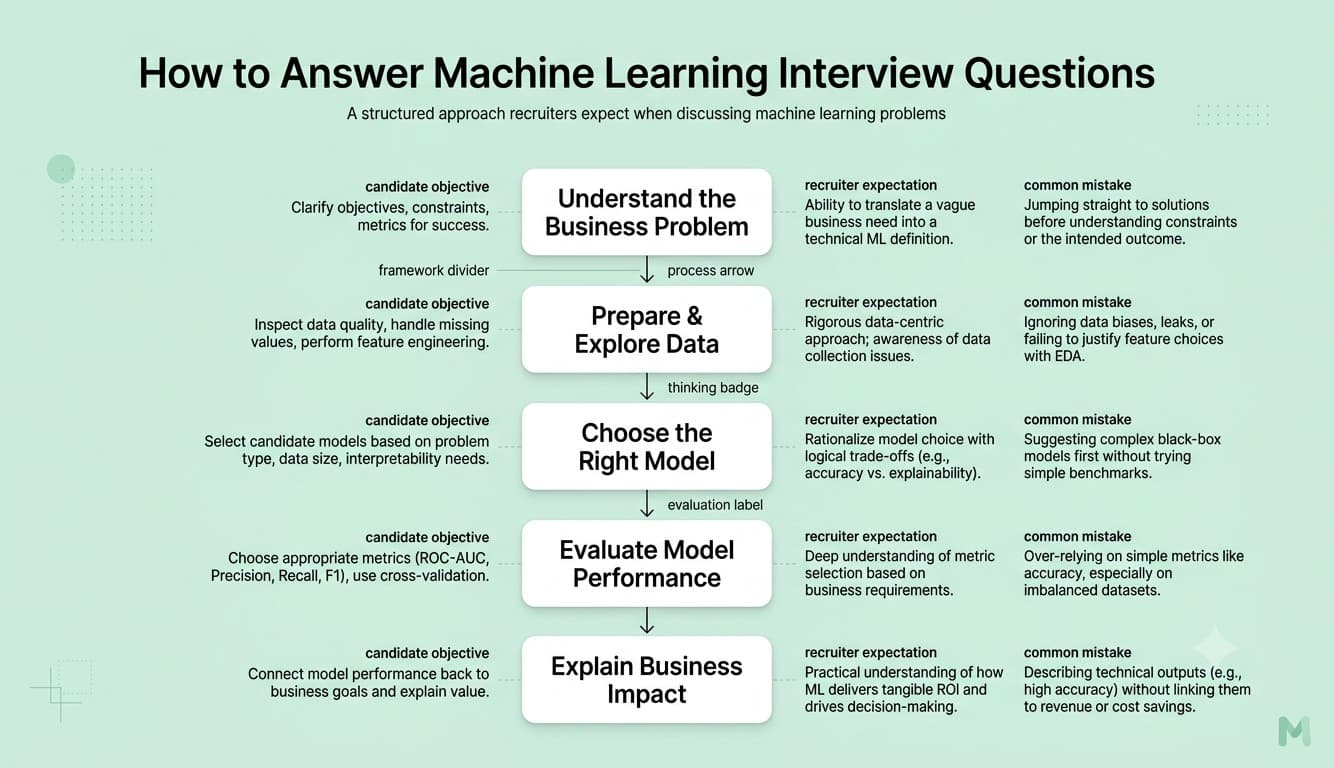
Question: What is the difference between supervised, unsupervised, and reinforcement learning?
Answer: Supervised learning trains a model on labeled data (input-output pairs) to predict outputs for new inputs (e.g., classification, regression). Unsupervised learning finds patterns/structure in unlabeled data without a specific target output (e.g., clustering, dimensionality reduction). Reinforcement learning trains an agent to take actions in an environment to maximize cumulative reward through trial-and-error interaction, rather than learning from a fixed labeled dataset.
Explanation: Foundational machine learning vocabulary, almost always asked early in a technical interview to establish baseline understanding.
Real-World Example: Predicting customer churn from labeled historical data (churned/not churned) is supervised learning; segmenting customers into behavioral groups without predefined labels is unsupervised learning; training a recommendation system that learns from user interactions and long-term engagement to optimize content sequencing is a reinforcement learning application.
Common Mistakes: Giving only the textbook definitions without concrete examples, or being unable to identify which category a specific described business problem falls into.
Follow-up Questions: Can you give an example of a semi-supervised learning scenario? How would you decide whether a business problem calls for supervised or unsupervised learning? What's self-supervised learning, and how does it differ from traditional unsupervised learning?
Question 17
Question: Explain how a decision tree works, and what criteria are used to split nodes.
Answer: A decision tree recursively splits the data into subsets based on feature values, choosing at each node the split that best separates the data according to a criterion — Gini impurity or entropy/information gain for classification, and variance reduction (typically mean squared error) for regression — continuing until a stopping condition (max depth, minimum samples per leaf) is reached.
Explanation: Decision trees underlie many powerful ensemble methods (random forests, gradient boosting), making a solid conceptual understanding foundational to much of applied machine learning.
Real-World Example: A credit approval decision tree might first split on income level, then within each income bracket split further on credit history length, producing an interpretable set of rules that a business/compliance team can review and understand directly, unlike many "black box" models.
Common Mistakes: Not being able to explain the actual splitting criterion mathematically (Gini impurity or entropy) beyond a vague "it finds the best split," or not mentioning that trees are prone to overfitting without constraints like max depth or pruning.
Follow-up Questions: What's the difference between Gini impurity and entropy as splitting criteria? How would you prevent a decision tree from overfitting? How does a decision tree handle missing values or categorical variables with many levels?
Question 18
Question: How does a random forest work, and why does it typically outperform a single decision tree?
Answer: A random forest builds many decision trees, each trained on a bootstrapped sample of the training data (bagging) and considering only a random subset of features at each split, then averages (regression) or votes (classification) across all trees for the final prediction. This reduces variance significantly compared to a single tree by decorrelating the individual trees' errors, while keeping bias relatively low, generally improving generalization.
Explanation: A very commonly used and tested ensemble method, testing understanding of how combining multiple weak/high-variance models can produce a stronger, more robust overall model.
Real-World Example: A random forest predicting loan default risk is generally more robust and accurate than a single decision tree, since it averages out the tendency of any individual tree to overfit to noise or idiosyncratic patterns in its specific training sample.
Common Mistakes: Not explaining both key sources of randomness (bootstrapped data sampling AND random feature subsetting at each split) — mentioning only one misses half the mechanism that makes random forests effective.
Follow-up Questions: What's the difference between bagging and boosting? How would you tune the number of trees and max features hyperparameters? How can you extract feature importance from a random forest, and what are the limitations of that importance measure?
Question 19
Question: Explain gradient boosting, and how does it differ from random forests?
Answer: Gradient boosting builds trees sequentially, where each new tree is trained to correct the errors (residuals, more precisely the gradient of the loss function) made by the ensemble of previous trees, gradually improving the overall model — unlike random forests, which build trees independently and in parallel via bagging. Boosting typically achieves lower bias than bagging-based methods but requires careful tuning (learning rate, number of trees, tree depth) to avoid overfitting.
Explanation: One of the most widely used and highest-performing model families in practice (XGBoost, LightGBM, CatBoost), making solid conceptual understanding essential for most applied data science roles.
Real-World Example: Many winning solutions in structured/tabular data machine learning competitions use gradient boosting (XGBoost or LightGBM) due to its strong out-of-the-box performance on tabular data, often outperforming random forests and even neural networks on this data type.
Common Mistakes: Confusing bagging and boosting as similar/interchangeable ensemble strategies, when they differ fundamentally in whether trees are built independently (bagging) or sequentially to correct prior errors (boosting).
Follow-up Questions: What is the learning rate hyperparameter in gradient boosting, and how does it affect the bias-variance tradeoff? How would you tune a gradient boosting model to prevent overfitting? What's the difference between XGBoost, LightGBM, and CatBoost at a high level?
Question 20
Question: How does logistic regression work, and why is it called "regression" despite being used for classification?
Answer: Logistic regression models the probability of a binary outcome using the logistic (sigmoid) function applied to a linear combination of input features, producing outputs bounded between 0 and 1 that can be interpreted as probabilities and thresholded into class predictions. It's called "regression" because it directly models a continuous quantity (the log-odds of the outcome) as a linear function of the predictors, even though the final application is typically classification.
Explanation: One of the most commonly used and interpretable classification models, and understanding the underlying linear-in-log-odds mechanism (versus just treating it as a black box) is frequently tested.
Real-World Example: A logistic regression model predicting loan default risk produces both a probability score (useful for risk-based pricing) and interpretable coefficients (showing how each feature, like income or credit history, affects the log-odds of default) — valued in regulated industries requiring model interpretability.
Common Mistakes: Not being able to explain the sigmoid function's role or the concept of log-odds, or confusing logistic regression's linear decision boundary limitation with the flexibility of more complex non-linear models.
Follow-up Questions: How would you interpret a specific logistic regression coefficient in terms of odds ratio? What loss function does logistic regression optimize (log-loss/cross-entropy), and why not use mean squared error instead? How would you handle a logistic regression problem with class imbalance?
Question 21
Question: What is regularization, and what's the difference between L1 (Lasso) and L2 (Ridge) regularization?
Answer: Regularization adds a penalty term to a model's loss function based on the magnitude of its coefficients, discouraging overly complex models and reducing overfitting. L1 (Lasso) regularization penalizes the sum of absolute coefficient values, which can shrink some coefficients exactly to zero (performing automatic feature selection). L2 (Ridge) regularization penalizes the sum of squared coefficient values, shrinking coefficients toward zero but rarely to exactly zero, generally more effective when many features contribute small but real effects.
Explanation: A core technique for combating overfitting, frequently tested both conceptually and in terms of practical tradeoffs between the two main variants.
Real-World Example: A regression model with hundreds of correlated features might use Lasso to automatically identify and retain only the most important subset of features, producing a simpler, more interpretable final model, whereas Ridge might be preferred when most features are believed to contribute at least a small genuine effect.
Common Mistakes: Not knowing that L1 specifically induces sparsity (zeroing out coefficients) while L2 does not, or not being able to explain why this happens geometrically/mathematically at even a conceptual level.
Follow-up Questions: What is Elastic Net, and why would you use it instead of pure L1 or L2? How would you choose the regularization strength (the penalty hyperparameter) in practice? How does regularization relate to the bias-variance tradeoff?
Question 22
Question: Explain how k-means clustering works, and what are its key limitations?
Answer: K-means iteratively assigns each data point to the nearest of k cluster centroids, then recalculates each centroid as the mean of its assigned points, repeating until assignments stabilize. Key limitations: it requires specifying k in advance, assumes roughly spherical, similarly-sized clusters (struggling with irregular shapes or very different cluster sizes/densities), is sensitive to initial centroid placement (often mitigated with k-means++ initialization), and is sensitive to outliers and feature scaling.
Explanation: One of the most commonly used and tested unsupervised learning algorithms, with interviewers frequently probing for awareness of its practical limitations, not just the mechanics.
Real-World Example: Customer segmentation based on purchasing behavior commonly uses k-means, but if segments are naturally irregular in shape or very different in size (e.g., one huge "typical customer" cluster and a few small niche clusters), k-means may not recover meaningful segments without careful preprocessing or an alternative algorithm.
Common Mistakes: Not mentioning the need to standardize/scale features before applying k-means (since it relies on distance calculations, unscaled features with different ranges can dominate the clustering), or not knowing any method for choosing an appropriate k (like the elbow method or silhouette score).
Follow-up Questions: How would you determine an appropriate value for k (elbow method, silhouette score)? How does k-means handle categorical variables, and what would you use instead if your data is largely categorical? What clustering algorithm would you use if you suspected clusters weren't roughly spherical (e.g., DBSCAN)?
Question 23
Question: What is Principal Component Analysis (PCA), and when would you use it?
Answer: PCA is a dimensionality reduction technique that transforms correlated features into a smaller set of uncorrelated components (principal components), ordered by the amount of variance in the original data they capture, allowing you to retain most of the informative variance while discarding lower-variance, often noisier dimensions.
Explanation: A very commonly used and tested technique for handling high-dimensional data, both to reduce computational cost/overfitting risk and to enable visualization of high-dimensional data in 2-3 dimensions.
Real-World Example: A dataset with hundreds of highly correlated financial indicators might be reduced to a handful of principal components capturing the vast majority of the original variance, simplifying downstream modeling and reducing overfitting risk from having too many correlated raw features.
Common Mistakes: Not mentioning that features should be standardized before PCA (since it's sensitive to feature scale), or treating the resulting principal components as if they retain the original features' direct, individual interpretability (they're linear combinations, generally harder to interpret directly).
Follow-up Questions: How would you decide how many principal components to retain? How would you interpret what a specific principal component represents? What's the difference between PCA and t-SNE/UMAP for dimensionality reduction, especially for visualization purposes?
Question 24
Question: What is the difference between bagging and boosting?
Answer: Bagging (bootstrap aggregating) trains multiple models independently and in parallel on different bootstrapped samples of the data, then combines their predictions (averaging or voting) primarily to reduce variance. Boosting trains models sequentially, with each new model specifically focused on correcting the errors of the previous ensemble, primarily to reduce bias — though modern boosting implementations also manage variance carefully through regularization.
Explanation: A very commonly tested ensemble learning distinction, since both approaches are foundational to widely-used, high-performing model families.
Real-World Example: Random forests (bagging) are often chosen for their robustness and ease of tuning with less risk of overfitting, while gradient boosting methods (like XGBoost) are often chosen when maximum predictive accuracy is the priority and there's time/expertise available for more careful hyperparameter tuning.
Common Mistakes: Describing the two approaches vaguely without clearly articulating that bagging trains models independently/in parallel (variance reduction) while boosting trains sequentially, with each step correcting prior errors (bias reduction).
Follow-up Questions: Why is boosting generally more prone to overfitting than bagging if not carefully tuned? Can you name a specific algorithm for each approach? How would you decide between a bagging-based versus boosting-based approach for a specific project?
Question 25
Question: How does a support vector machine (SVM) work, and what is the "kernel trick"?
Answer: An SVM finds the hyperplane that maximally separates classes with the largest possible margin between the closest points of each class (support vectors). The kernel trick allows an SVM to implicitly map data into a higher-dimensional space where a linear separation becomes possible, without ever explicitly computing the (potentially very expensive) transformation, using a kernel function (like RBF or polynomial) to compute the necessary similarity/distance calculations directly in the original space.
Explanation: Tests understanding of a once-dominant, still-relevant classical ML method, particularly the kernel trick concept which reflects a broader, elegant computational technique.
Real-World Example: An SVM with an RBF kernel can effectively separate classes with a non-linear, circular decision boundary in the original feature space, something a simple linear model couldn't achieve, without the computational cost of explicitly transforming data into a much higher-dimensional space.
Common Mistakes: Not being able to explain the kernel trick's core insight (avoiding explicit high-dimensional transformation) beyond a vague "it makes things non-linear," or not knowing that SVMs are sensitive to feature scaling.
Follow-up Questions: How would you choose between a linear and RBF kernel for a given problem? How does the regularization parameter C affect the SVM's margin and overfitting risk? How does SVM performance and training time scale with dataset size, and what does that imply about when to use it?
Question 26
Question: What is the difference between generative and discriminative models?
Answer: Generative models learn the joint probability distribution of the features and labels, P(X, Y), enabling them to generate new synthetic data resembling the training distribution and, via Bayes' theorem, also perform classification. Discriminative models directly learn the decision boundary or conditional probability P(Y|X) without modeling how the features themselves were generated, generally requiring less data and fewer assumptions to achieve strong classification performance specifically.
Explanation: A conceptual distinction increasingly relevant given the prominence of generative AI, testing whether a candidate understands this fundamental modeling philosophy difference.
Real-World Example: Naive Bayes is a generative classifier (modeling how features are distributed within each class), while logistic regression is discriminative (directly modeling the decision boundary) — both can be used for the same classification task but rest on different underlying assumptions and offer different capabilities (e.g., only the generative model can generate new synthetic samples).
Common Mistakes: Confusing "generative" in this classical ML sense with generative AI/large language models specifically, without recognizing the term has a broader, longer-standing statistical meaning.
Follow-up Questions: Can you give another example pair of generative and discriminative models for the same task? Why do discriminative models often outperform generative ones on pure classification accuracy, given enough data? How does this distinction relate to modern generative AI models like GANs or diffusion models?
Question 27
Question: How would you handle a machine learning problem with severe class imbalance?
Answer: Approaches include resampling techniques (oversampling the minority class via SMOTE, or undersampling the majority class), adjusting class weights within the model's loss function to penalize misclassifying the minority class more heavily, choosing evaluation metrics appropriate for imbalance (precision, recall, F1, AUC-PR rather than raw accuracy), and considering anomaly-detection framings if the imbalance is extreme.
Explanation: An extremely common and practically important real-world scenario (fraud, churn, rare disease detection), testing awareness of both technique options and why standard accuracy is misleading in this context.
Real-World Example: A fraud detection model trained on data where only 0.1% of transactions are fraudulent would achieve 99.9% accuracy by trivially predicting "not fraud" for everything — clearly useless — requiring class weighting, resampling, and appropriate metrics like recall and precision to build a genuinely useful model.
Common Mistakes: Relying on raw accuracy as the primary evaluation metric for a severely imbalanced problem, which can be highly misleading and mask a model that's essentially useless for the minority class of actual interest.
Follow-up Questions: What's the difference between SMOTE and simple random oversampling? How would you choose an appropriate classification threshold for an imbalanced problem, rather than the default 0.5? How would you communicate the tradeoff between precision and recall to a business stakeholder for this kind of problem?
Question 28
Question: What is the curse of dimensionality, and how does it affect machine learning models?
Answer: As the number of features (dimensions) grows, the volume of the feature space grows exponentially, causing data points to become increasingly sparse and distances between points to become less meaningful — this degrades the performance of distance-based methods (like k-NN or k-means), increases the risk of overfitting (since more features increase model flexibility relative to a fixed amount of data), and generally requires exponentially more data to maintain the same statistical density/reliability as dimensionality grows.
Explanation: A foundational conceptual challenge underlying the motivation for dimensionality reduction and feature selection techniques, frequently tested to gauge deeper intuition about high-dimensional data behavior.
Real-World Example: A k-nearest-neighbors model that works well with 5 meaningful features might perform poorly with 500 sparse, mostly-irrelevant features, since "nearest neighbor" distances become increasingly uniform and uninformative in very high-dimensional spaces.
Common Mistakes: Not being able to explain the specific mechanism (data sparsity, distance concentration) behind the curse of dimensionality beyond a vague "more features are bad."
Follow-up Questions: How does the curse of dimensionality specifically affect distance-based algorithms like k-NN? What techniques would you use to combat the curse of dimensionality? Does the curse of dimensionality affect tree-based models (like random forests) the same way it affects distance-based models?
Question 29
Question: How would you approach feature selection for a machine learning model with a very large number of candidate features?
Answer: Approaches include filter methods (statistical tests or correlation with the target, computed independently of any model, fast but ignoring feature interactions), wrapper methods (iteratively adding/removing features based on actual model performance, like recursive feature elimination, more accurate but computationally expensive), and embedded methods (feature selection built into the model training process itself, like Lasso regularization or tree-based feature importance, balancing accuracy and efficiency).
Explanation: A very practical, commonly tested question since real-world datasets often have far more candidate features than are useful or computationally efficient to include.
Real-World Example: A model with thousands of candidate marketing/behavioral features might use Lasso regularization (an embedded method) to automatically identify and retain only the most predictive subset, both improving generalization and producing a more interpretable, maintainable final model.
Common Mistakes: Selecting features using only a simple univariate correlation check with the target, missing potentially important features that only matter in combination with other features (interaction effects).
Follow-up Questions: What's the risk of doing feature selection using the entire dataset (including the test set) before splitting into train/test? How would you handle feature selection differently for a tree-based model versus a linear model? How do you balance interpretability against predictive performance when deciding how aggressively to reduce the feature set?
Question 30
Question: What is transfer learning, and when is it useful?
Answer: Transfer learning takes a model pretrained on a large, related dataset/task and adapts (fine-tunes) it for a new, often smaller, related task, leveraging previously learned general representations rather than training a new model entirely from scratch — particularly valuable when labeled data for the new task is limited, since the pretrained model already captures broadly useful patterns.
Explanation: An increasingly important concept, especially in deep learning, testing awareness of a technique that dramatically reduces data and compute requirements for many real-world applications.
Real-World Example: A company building an image classifier to detect specific defective products on a manufacturing line, with only a few thousand labeled images available, would typically fine-tune a large image model pretrained on millions of general images, rather than training a new convolutional network entirely from scratch, dramatically improving performance given the limited labeled data available.
Common Mistakes: Attempting to train a large, complex model entirely from scratch on a small, task-specific dataset when a pretrained model fine-tuned for the task would likely perform significantly better with far less data and compute.
Follow-up Questions: How would you decide how many layers to freeze versus fine-tune when adapting a pretrained model? What's the difference between feature extraction and fine-tuning as transfer learning strategies? What risks arise if the pretrained model's original training data is very different (domain mismatch) from your new task's data?
Part 3: Model Evaluation & Validation
Question 31
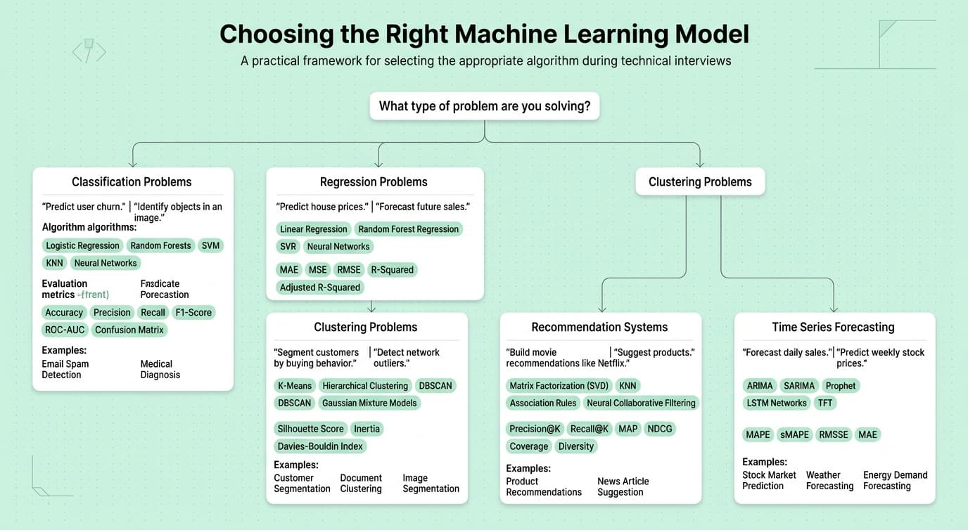
Question: What's the difference between precision and recall, and when would you prioritize one over the other?
Answer: Precision measures the proportion of positive predictions that are actually correct (minimizing false positives), while recall measures the proportion of actual positives that the model correctly identifies (minimizing false negatives). Prioritization depends on the relative cost of each error type in the specific business context — high-stakes situations where missing a positive is costly favor recall, while situations where false positives are costly favor precision.
Explanation: One of the most fundamental and frequently tested model evaluation concepts, since choosing the wrong metric to optimize can lead to a model that's technically accurate but practically useless for the business need.
Real-World Example: A cancer screening model should prioritize recall (minimizing missed diagnoses, even at the cost of more false alarms requiring follow-up testing), while a spam filter should prioritize precision (minimizing legitimate emails incorrectly flagged as spam, even if some spam gets through).
Common Mistakes: Optimizing for overall accuracy without considering the specific, differing costs of false positives versus false negatives for the actual business problem at hand.
Follow-up Questions: What is the F1 score, and when would you use it instead of looking at precision and recall separately? How would you choose a classification threshold to balance precision and recall appropriately for a specific use case? Can you draw or describe a precision-recall curve and explain what it shows?
Question 32
Question: Explain the ROC curve and AUC. What are their limitations?
Answer: A ROC (Receiver Operating Characteristic) curve plots the true positive rate against the false positive rate across all possible classification thresholds, and AUC (Area Under the Curve) summarizes this into a single number representing the model's ability to rank positive examples higher than negative ones, regardless of a specific threshold. A key limitation: AUC can be misleadingly optimistic on highly imbalanced datasets, since it's insensitive to the actual class distribution — in those cases, a Precision-Recall curve/AUC-PR is often more informative.
Explanation: A very commonly used and tested classification evaluation metric, with interviewers often specifically probing for awareness of its imbalanced-data limitation, since this is a very common real-world pitfall.
Real-World Example: A fraud detection model with 0.5% fraud prevalence might show a deceptively high AUC-ROC (e.g., 0.95) while still performing poorly in practice on the metric that actually matters (precision at a usable recall level) — AUC-PR would more clearly reveal this weaker real-world performance.
Common Mistakes: Reporting AUC-ROC as the sole evaluation metric for a highly imbalanced classification problem without considering the more informative AUC-PR or examining the confusion matrix at a realistic operating threshold.
Follow-up Questions: Why is AUC-PR often more informative than AUC-ROC for imbalanced datasets? How would you explain AUC to a non-technical stakeholder? What does an AUC of 0.5 mean, and what would an AUC below 0.5 imply?
Question 33
Question: What is cross-validation, and why is it used instead of a single train/test split?
Answer: Cross-validation (commonly k-fold) splits the data into k subsets, training on k-1 folds and validating on the remaining fold, repeating this k times so every observation serves as validation data exactly once, then averaging the resulting performance metrics — this provides a more robust, less variance-prone estimate of model performance than a single, potentially lucky or unlucky, train/test split.
Explanation: A foundational model validation technique, essential for reliable model selection and hyperparameter tuning, frequently tested since misuse (like data leakage between folds) is a common real-world mistake.
Real-World Example: Comparing two candidate models using a single train/test split might show one performing better purely due to chance in how that particular split happened to fall, while 5-fold cross-validation averaged across multiple different splits gives a much more reliable basis for choosing between them.
Common Mistakes: Performing preprocessing steps (like scaling, or feature selection) using the entire dataset before cross-validation splitting, causing data leakage between folds and an overly optimistic performance estimate.
Follow-up Questions: How would you adapt standard k-fold cross-validation for time-series data, where random shuffling would violate temporal order? What's the difference between k-fold and stratified k-fold cross-validation, and when would you need the latter? How would you choose an appropriate value for k?
Question 34
Question: How would you detect and address overfitting in a machine learning model?
Answer: Detection: compare training versus validation/test performance — a large gap (strong training performance, much weaker validation performance) indicates overfitting; learning curves showing validation error diverging from training error as training progresses are another clear signal. Addressing it: gather more training data, simplify the model (fewer features/parameters, shallower trees), apply regularization, use cross-validation for more reliable model selection, or apply early stopping (for iterative models like neural networks or gradient boosting).
Explanation: One of the most fundamental practical machine learning skills, testing both diagnostic ability and a concrete toolkit of remediation techniques.
Real-World Example: A deep decision tree achieving 99% accuracy on training data but only 70% on validation data is a clear overfitting signal, addressable by limiting tree depth, requiring a higher minimum samples per leaf, or switching to a regularized ensemble method like a random forest.
Common Mistakes: Only looking at training performance when evaluating a model, never comparing against a held-out validation/test set, missing overfitting entirely until the model performs poorly in production.
Follow-up Questions: How would you distinguish overfitting from a genuinely difficult, high-noise problem where even a well-fit model has limited accuracy? What's the difference between early stopping and regularization as overfitting remedies? How would you use a learning curve to diagnose whether more training data would actually help?
Question 35
Question: How would you validate a machine learning model for a time-series forecasting problem?
Answer: Use time-based (walk-forward or rolling-origin) validation rather than standard random k-fold cross-validation, since randomly shuffling time-series data would allow the model to "see the future" when predicting the past, causing data leakage and an unrealistically optimistic performance estimate — train on data up to a point in time, validate on the immediately following period, then roll the window forward and repeat.
Explanation: A very commonly tested pitfall specific to time-series problems, since standard cross-validation techniques (appropriate for i.i.d. data) are inappropriate and can produce badly misleading results if applied naively.
Real-World Example: Validating a sales forecasting model using standard random k-fold cross-validation could allow the model to be trained on data from a later month while being validated on an earlier month, letting future information (like a since-discovered market trend) leak backward — a walk-forward validation scheme prevents this by always respecting temporal order.
Common Mistakes: Applying standard random cross-validation to time-series data without considering the temporal ordering, resulting in data leakage and overly optimistic validation performance that fails to hold up in real, live forecasting.
Follow-up Questions: How would you handle seasonality when validating a time-series model? What is data leakage more broadly, and can you give another example of it beyond the time-series case? How would you choose an appropriate size for the rolling training window?
Question 36
Question: What is a confusion matrix, and what metrics can you derive from it?
Answer: A confusion matrix is a table showing the counts of true positives, true negatives, false positives, and false negatives for a classification model's predictions against actual outcomes. From it, you can derive accuracy (overall correct rate), precision (true positives / predicted positives), recall (true positives / actual positives), specificity (true negatives / actual negatives), and F1 score (harmonic mean of precision and recall).
Explanation: A very foundational classification evaluation concept, essential vocabulary underlying most classification metric discussions.
Real-World Example: Reviewing a fraud model's confusion matrix might reveal it has high overall accuracy but a concerning number of false negatives (missed actual fraud cases) — a nuance that a single "accuracy" number alone would completely hide.
Common Mistakes: Only reporting overall accuracy without examining the full confusion matrix, missing important nuances about specific error types that matter more for the business (like false negatives in a high-stakes detection problem).
Follow-up Questions: How would a confusion matrix look different for a highly imbalanced dataset even for a fairly good model? How would you extend a confusion matrix to a multi-class classification problem? How would you use a confusion matrix to decide whether to adjust a model's classification threshold?
Question 37
Question: What evaluation metrics would you use for a regression problem, and what are their tradeoffs?
Answer: Mean Absolute Error (MAE) measures average absolute prediction error, robust to outliers and easily interpretable in the original units. Mean Squared Error (MSE) penalizes larger errors disproportionately more (squared), useful when large errors are especially costly, but sensitive to outliers. Root Mean Squared Error (RMSE) returns MSE to the original units for interpretability. R-squared measures the proportion of variance in the target explained by the model, useful for a relative sense of fit but can be misleading in isolation without also examining absolute error magnitude.
Explanation: A foundational regression evaluation question testing whether a candidate can match the right metric to the specific business tolerance for large versus small errors.
Real-World Example: A demand forecasting model where being off by a large amount on any single day is especially costly (e.g., causing stockouts) might prioritize minimizing RMSE (penalizing large errors more), while a model where consistent moderate accuracy matters more than occasional large misses might prioritize MAE.
Common Mistakes: Reporting only R-squared without also examining absolute error metrics (MAE/RMSE) in the original, business-meaningful units, which can obscure whether the actual magnitude of errors is acceptable for the use case.
Follow-up Questions: When would you prefer MAE over RMSE, and vice versa? What's a limitation of R-squared as a standalone metric, especially for comparing models with different numbers of features? How would you communicate a regression model's expected error to a non-technical stakeholder?
Question 38
Question: How would you decide on a classification threshold rather than using the default 0.5?
Answer: Analyze the precision-recall tradeoff across different threshold values (using a precision-recall curve), and select a threshold based on the specific business cost of false positives versus false negatives — for example, using a cost-weighted approach that explicitly quantifies the dollar (or other) cost of each error type and selects the threshold minimizing total expected cost, rather than defaulting to an arbitrary 0.5 cutoff that has no inherent business meaning.
Explanation: A very practical, frequently tested applied question, since the default 0.5 threshold is rarely actually optimal for the real business objective at hand.
Real-World Example: A model flagging potentially fraudulent transactions for manual review might use a much lower threshold than 0.5 if the cost of a missed fraud case (a false negative) is far higher than the cost of an unnecessary manual review (a false positive).
Common Mistakes: Defaulting to the standard 0.5 threshold without any deliberate consideration of the actual relative costs of the two error types for the specific business problem.
Follow-up Questions: How would you quantify the cost of a false positive versus a false negative for a specific business scenario? How would changing the threshold over time (e.g., seasonally) be justified or not? How would you communicate a threshold decision and its tradeoffs to a business stakeholder?
Question 39
Question: What is data leakage, and how would you detect and prevent it in a machine learning pipeline?
Answer: Data leakage occurs when information from outside the legitimate training dataset (often information that wouldn't be available at actual prediction time) inadvertently influences model training, causing artificially inflated validation performance that fails to hold up in real-world deployment. Prevention: carefully audit feature engineering for any use of future or target-derived information, ensure preprocessing steps (scaling, imputation, feature selection) are fit only on training data and then applied to validation/test data, and use appropriate time-aware splitting for temporal data.
Explanation: One of the most consequential and commonly tested practical pitfalls in machine learning, since leakage often produces a model that looks excellent in validation but performs poorly or fails outright in production.
Real-World Example: A model predicting hospital readmission that accidentally includes a "discharge disposition" feature (which is only known after the outcome being predicted has essentially already occurred) would show unrealistically strong validation performance that collapses once deployed, since that information isn't genuinely available at prediction time.
Common Mistakes: Not carefully considering whether each feature would actually be available and known at the real moment of prediction in production, only discovering the leakage after a suspiciously high-performing model fails to replicate its performance once deployed.
Follow-up Questions: Can you give another concrete example of data leakage you've encountered or could imagine? How would you specifically audit a feature engineering pipeline for potential leakage? What's target leakage specifically, and how does it differ from other forms of leakage (like train/test contamination)?
Question 40
Question: How would you evaluate whether a machine learning model is ready for production deployment?
Answer: Beyond standard offline evaluation metrics (accuracy, precision/recall, RMSE, etc.), consider: performance stability across relevant subgroups/segments (not just in aggregate), robustness to realistic data quality issues and edge cases, latency/computational cost requirements for the production serving environment, a clear plan for ongoing monitoring (performance and data drift), and, ideally, a controlled rollout (like a shadow deployment or a small-scale A/B test) to validate real-world performance before a full launch.
Explanation: A holistic, practically-oriented question testing whether a candidate thinks beyond a single offline metric toward the full lifecycle considerations of responsibly deploying a model.
Real-World Example: A model with strong aggregate accuracy might still perform poorly for a specific important subgroup (e.g., a particular customer segment or region) — a shadow deployment comparing the new model's live predictions against the current production system's, without yet acting on them, can catch this kind of issue before a risky full launch.
Common Mistakes: Treating a strong offline validation metric as sufficient justification for deployment without considering subgroup performance, latency constraints, or a plan for post-launch monitoring.
Follow-up Questions: How would you design a shadow deployment or canary rollout for a new model? What ongoing monitoring would you put in place after deployment to catch model or data drift? How would you decide whether a model's performance on a specific important subgroup is acceptable, even if aggregate performance looks strong?
Part 4: Feature Engineering & Data Preprocessing
Question 41
Question: How would you handle missing data before training a machine learning model?
Answer: Options depend on the missingness mechanism and extent: drop rows/columns if missingness is minimal and random, impute with a statistic (mean/median/mode) or a more sophisticated model-based approach (like k-NN imputation or iterative imputation) for moderate missingness, or create a separate "missing" indicator feature if the fact that a value is missing might itself carry predictive signal — and critically, fit any imputation strategy only on training data to avoid leakage into validation/test sets.
Explanation: A very commonly tested practical preprocessing question, since virtually every real-world dataset has missing values requiring a deliberate, justified handling strategy.
Real-World Example: In a customer dataset, a missing "income" value might be imputed with a segment-specific median, while also adding a binary "income_was_missing" feature, since the fact that a customer didn't provide income information might itself be predictive of certain behaviors.
Common Mistakes: Applying a single blanket imputation strategy (like always using the overall mean) without considering whether missingness might vary meaningfully by subgroup, or whether missingness itself might carry useful signal.
Follow-up Questions: How would you decide between simple imputation and a more sophisticated model-based imputation approach? How does the missing data mechanism (missing completely at random vs. missing not at random) affect your chosen strategy? How would you handle missing data differently for a tree-based model versus a linear model?
Question 42
Question: What is feature scaling, and when is it necessary?
Answer: Feature scaling transforms features to a common scale (e.g., standardization to zero mean and unit variance, or min-max normalization to a fixed range), necessary for algorithms sensitive to feature magnitude and distance calculations (like k-NN, SVM, gradient descent-based methods including neural networks and linear/logistic regression), but generally unnecessary for tree-based models (decision trees, random forests, gradient boosting), which split based on feature order/thresholds rather than magnitude.
Explanation: A very commonly tested practical concept, since applying (or failing to apply) scaling appropriately is a frequent source of both errors and unnecessary extra work.
Real-World Example: A k-NN model using both "age" (range roughly 0-100) and "income" (range potentially 0-500,000) without scaling would have distance calculations almost entirely dominated by the income feature simply due to its much larger raw numeric range, regardless of its actual relative importance.
Common Mistakes: Applying scaling unnecessarily to tree-based models (harmless but wasted effort), or forgetting to apply scaling for models that genuinely require it (like k-NN, SVM, or neural networks), leading to a feature's raw scale disproportionately dominating the model.
Follow-up Questions: What's the difference between standardization and normalization/min-max scaling, and when would you choose one over the other? How would you correctly apply scaling within a cross-validation pipeline to avoid data leakage? Does scaling affect a model's interpretability or just its optimization/performance?
Question 43
Question: How would you encode categorical variables for a machine learning model?
Answer: Common approaches: one-hot encoding (creating a binary column per category, suitable for nominal categories with a reasonable number of levels, but can cause a dimensionality explosion with high-cardinality features), label/ordinal encoding (assigning integers, appropriate only when categories have a genuine inherent order), and target/mean encoding (replacing each category with a statistic of the target variable for that category, powerful for high-cardinality features but requires careful regularization/cross-validation to avoid leakage and overfitting).
Explanation: A very commonly tested practical preprocessing skill, testing whether a candidate matches the encoding method to the categorical variable's specific characteristics (cardinality, whether there's genuine order).
Real-World Example: A "zip code" feature with thousands of unique values would create an unwieldy number of columns with one-hot encoding, making target encoding (or a learned embedding, in deep learning contexts) a more practical choice, while a small, low-cardinality "shirt size" (S/M/L/XL) feature with genuine order is well suited to ordinal encoding.
Common Mistakes: Using label/ordinal encoding for a nominal (non-ordered) categorical variable, which incorrectly implies a false numeric ordering/distance relationship between category values that the model may inadvertently learn from.
Follow-up Questions: What's the risk of target encoding causing data leakage, and how would you mitigate it (e.g., with cross-validation-based encoding)? How would you handle a categorical feature with a category that appears in the test set but not the training set? How does the choice of encoding differ for tree-based versus linear models?
Question 44
Question: What is feature engineering, and can you give an example of creating a valuable engineered feature from raw data?
Answer: Feature engineering is the process of using domain knowledge to create new input features from raw data that better expose the underlying patterns relevant to the prediction task, often having a larger impact on model performance than the specific choice of algorithm.
Explanation: A very commonly tested, open-ended question assessing creativity and domain-application skill beyond purely technical/algorithmic knowledge — often considered one of the highest-leverage skills in applied data science.
Real-World Example: For a churn prediction model, rather than using only raw "last login date," engineering a "days since last login" feature (and further, a "trend in login frequency over the last 30 days" feature) often captures much more predictive signal about disengagement than the raw timestamp alone.
Common Mistakes: Relying entirely on raw features "as-is" without applying domain knowledge to construct more informative derived features, leaving significant predictive power on the table that a more thoughtful feature engineering process would have captured.
Follow-up Questions: Can you walk through your feature engineering process for a project you've worked on? How would you avoid creating a feature that inadvertently causes data leakage? How would you evaluate whether a newly engineered feature is actually adding value to the model?
Question 45
Question: How would you detect and handle outliers before or during model training?
Answer: Detection methods include visual inspection (box plots, scatter plots), statistical thresholds (values beyond 1.5x IQR from the quartiles, or several standard deviations from the mean), and model-based approaches (like isolation forests for multivariate outlier detection). Handling depends on the cause: correct clear data entry errors, consider removing or capping (winsorizing) genuine extreme values if they're likely to unduly distort model training, or use robust modeling techniques/loss functions less sensitive to outliers if the extreme values are legitimate and shouldn't simply be discarded.
Explanation: A practical data preprocessing skill, testing thoughtful judgment (not a reflexive "always remove outliers" approach) about the cause and appropriate handling of extreme values.
Real-World Example: In a dataset of customer order values, a $1 million order might be a legitimate large B2B transaction (should likely be retained, perhaps analyzed or modeled separately from typical consumer transactions) or a data entry error (should be corrected) — the appropriate handling depends entirely on investigation.
Common Mistakes: Automatically removing all statistical outliers without investigating whether they represent genuine, important data points (like real high-value customers) versus actual errors.
Follow-up Questions: How would outlier handling differ for a linear regression model versus a tree-based model (which is generally more robust to outliers)? What is winsorizing, and how does it differ from simply removing outliers? How would you detect multivariate outliers that might not appear extreme on any single feature individually?
Question 46
Question: How would you handle a situation where your training data isn't representative of the population you'll actually make predictions on in production (covariate shift)?
Answer: First detect it by comparing feature distributions between training data and current production/live data (using statistical tests or visualization), then consider mitigation strategies: reweighting training samples to better match the target production distribution, collecting additional, more representative training data, or retraining the model more frequently to keep pace with a distribution that's genuinely evolving over time.
Explanation: An important, increasingly tested real-world robustness concept, since training/production data mismatches are a very common and often silent cause of model performance degradation.
Real-World Example: A model trained primarily on pre-pandemic e-commerce purchasing behavior might perform poorly when deployed on significantly shifted post-pandemic purchasing patterns, requiring detection of this covariate shift and either retraining on more recent, representative data or reweighting to better reflect current patterns.
Common Mistakes: Assuming a model's strong offline validation performance (evaluated on data that mirrors the training distribution) will automatically hold up in production without checking whether production data has meaningfully drifted from the training data's characteristics.
Follow-up Questions: What statistical techniques would you use to detect covariate shift between training and production data? How would you decide how frequently to retrain a model given data that evolves over time? What's the difference between covariate shift and concept drift?
Question 47
Question: How would you engineer features from time-series or temporal data?
Answer: Common techniques include: lag features (past values of a variable at various time offsets), rolling window statistics (rolling mean, standard deviation, min/max over a recent window), time-based features (day of week, month, holiday indicators to capture seasonality), and rate-of-change/trend features (e.g., percentage change over the last week) — all while being careful to compute these features using only information that would genuinely have been available at each historical point in time, to avoid leakage.
Explanation: A practically important skill for the very common category of business problems involving time-ordered data, testing both feature creativity and leakage-awareness specific to temporal data.
Real-World Example: A demand forecasting model might use a 7-day rolling average of past sales, an indicator for whether the current date is a holiday, and the sales figure from exactly one year prior (to capture annual seasonality) as engineered features, each carefully computed to only use information available up to that point in time.
Common Mistakes: Accidentally using a rolling window or aggregate statistic that includes future data points relative to the specific row/timestamp being predicted, introducing subtle data leakage that inflates offline validation performance unrealistically.
Follow-up Questions: How would you handle multiple overlapping seasonal patterns (e.g., both weekly and yearly seasonality) in your feature engineering? How would you validate that your time-based features don't contain any leakage? How would you engineer features to capture a trend that might be changing/accelerating over time?
Question 48
Question: What is the difference between dimensionality reduction for feature engineering versus for visualization, and how does that affect your technique choice?
Answer: For feature engineering/modeling purposes, dimensionality reduction (like PCA) aims to preserve as much of the informative variance as possible in a computationally efficient, often linear transformation, prioritizing downstream model performance. For visualization purposes, techniques like t-SNE or UMAP prioritize preserving local neighborhood structure and producing visually interpretable, well-separated clusters in 2-3 dimensions, even at the cost of not preserving global distances as faithfully as PCA — making them excellent for visual exploration but generally less suitable as direct inputs to a downstream predictive model.
Explanation: Tests nuanced understanding that "dimensionality reduction" isn't a single interchangeable technique — the right choice depends specifically on whether the end goal is modeling or human visual interpretation.
Real-World Example: A data scientist might use PCA to reduce a high-dimensional customer feature set before feeding it into a clustering model (preserving overall variance structure for the algorithm), but then use t-SNE or UMAP specifically to create a compelling 2D visualization of those resulting clusters for a stakeholder presentation.
Common Mistakes: Using t-SNE or UMAP output as direct input features into a downstream predictive model (their non-linear, locally-focused transformations aren't well suited to this purpose and their output can be unstable/non-deterministic across runs), rather than reserving them specifically for visualization.
Follow-up Questions: Why is t-SNE generally unsuitable as a preprocessing step for a downstream predictive model? How would you interpret the axes of a t-SNE or UMAP plot (and what's a common misinterpretation to avoid)? How does UMAP differ from t-SNE in terms of preserving global versus local structure?
FREE TO USE
8k+ SESSIONS92% FLUENCY4.9★ RATING
Speak With Confidence
Real Conversations. Real Scenarios. Speak until it feels natural.
- Real-Time Speaking Practice
- Guided Conversation Flows
- Instant AI Feedback
Part 5: Deep Learning & Neural Networks
Question 49
Question: Explain how backpropagation works in training a neural network.
Answer: Backpropagation computes the gradient of the loss function with respect to each weight in the network by applying the chain rule of calculus, propagating the error backward from the output layer through each hidden layer to the input layer — these gradients are then used by an optimization algorithm (like gradient descent) to update each weight in the direction that reduces the loss.
Explanation: The foundational algorithm underlying how virtually all neural networks are trained, and a very commonly tested concept to gauge whether a candidate understands the mechanics beneath the "black box" of deep learning frameworks.
Real-World Example: Every time a deep learning framework like PyTorch or TensorFlow calls .backward() or computes gradients during training, it's performing automatic differentiation implementing the backpropagation algorithm under the hood, whether for an image classifier or a large language model.
Common Mistakes: Being able to describe backpropagation only vaguely ("it adjusts the weights based on the error") without connecting it to the specific mechanism of the chain rule propagating gradients layer by layer backward through the network.
Follow-up Questions: What is the vanishing gradient problem, and how does it relate to backpropagation in deep networks? How does backpropagation differ between a feedforward network and a recurrent neural network (backpropagation through time)? What role does the learning rate play in how gradients are used to update weights?
Question 50
Question: What is the vanishing/exploding gradient problem, and how is it addressed in modern deep learning?
Answer: In deep networks, gradients can become extremely small (vanishing) or extremely large (exploding) as they're propagated backward through many layers during backpropagation, especially with certain activation functions (like sigmoid/tanh) — this makes training very deep networks difficult, as early layers either barely update (vanishing) or become unstable (exploding). Modern solutions include using ReLU-family activation functions (which don't saturate for positive inputs), careful weight initialization schemes (like He or Xavier initialization), batch normalization, gradient clipping (for exploding gradients), and architectural innovations like residual/skip connections (as in ResNets and Transformers).
Explanation: A foundational deep learning challenge and a very commonly tested question, since understanding this problem motivates many of the standard architectural and training choices used in modern neural networks.
Real-World Example: Training very deep convolutional networks became practical largely due to residual connections (introduced in ResNet), which provide a more direct path for gradients to flow backward through the network, substantially mitigating the vanishing gradient problem that had previously limited how deep networks could effectively be trained.
Common Mistakes: Not connecting the problem to specific, concrete architectural or training solutions (like ReLU, batch norm, or residual connections), giving only an abstract description of the problem without practical remediation knowledge.
Follow-up Questions: Why does the ReLU activation function help mitigate the vanishing gradient problem compared to sigmoid? What is gradient clipping, and specifically how does it address exploding gradients? How do residual/skip connections help gradients flow more effectively through very deep networks?
Question 51
Question: What is the difference between a Convolutional Neural Network (CNN) and a Recurrent Neural Network (RNN), and what data types is each suited for?
Answer: CNNs use convolutional filters that slide across input data to detect local, spatially-invariant patterns, making them especially well suited for grid-like data such as images (detecting edges, textures, and higher-level visual patterns hierarchically). RNNs process sequential data one step at a time while maintaining an internal hidden state that carries information forward through the sequence, making them (historically) well suited for sequential/temporal data like text or time series, though largely superseded by Transformer architectures for many sequential tasks today.
Explanation: A foundational architectural distinction, testing whether a candidate can match network architecture to the underlying structure of the input data.
Real-World Example: Image classification tasks (identifying objects in photos) are a natural fit for CNNs, which exploit spatial locality, while, historically, tasks like language translation used RNNs (and their gated variants like LSTM/GRU) to process word sequences, though modern language models have largely shifted to Transformer architectures instead.
Common Mistakes: Not being able to explain why CNNs are particularly well suited to spatial/grid data specifically (parameter sharing via convolution, translation invariance), or not being aware that Transformers have largely superseded RNNs for most modern sequential/language tasks.
Follow-up Questions: What problem do LSTM and GRU architectures solve relative to a basic (vanilla) RNN? Why have Transformers largely replaced RNNs for many sequential modeling tasks? How does a CNN's use of parameter sharing (the same filter applied across the whole image) contribute to its efficiency and effectiveness?
Question 52
Question: Explain the Transformer architecture and the role of the self-attention mechanism.
Answer: The Transformer architecture processes an entire sequence in parallel (rather than step-by-step like an RNN), using a self-attention mechanism that allows each position in the sequence to directly weigh and incorporate information from every other position, dynamically learning which parts of the input are most relevant to each other — this enables both much better parallelization during training (compared to sequential RNN processing) and more effective modeling of long-range dependencies in the data.
Explanation: A very current and increasingly essential architecture to understand given its role underlying nearly all modern large language models, making this an increasingly commonly tested concept even for data scientists not specifically in NLP-focused roles.
Real-World Example: Modern large language models (like GPT-family and other LLMs) are built on the Transformer architecture, whose self-attention mechanism allows the model to correctly resolve, for example, which earlier noun a pronoun like "it" refers to in a long, complex sentence — a task that's difficult for older, purely sequential RNN-based architectures to handle reliably over long distances.
Common Mistakes: Being able to name "attention" as a component without being able to explain the core intuition (each token dynamically attending to/weighing relevant other tokens) or why this specifically enables better parallelization and long-range dependency modeling compared to RNNs.
Follow-up Questions: What is multi-head attention, and why use multiple attention heads rather than just one? How does positional encoding address the fact that self-attention alone has no inherent sense of sequence order? What's the difference between an encoder-only, decoder-only, and encoder-decoder Transformer architecture?
Question 53
Question: What is dropout, and how does it help prevent overfitting in neural networks?
Answer: Dropout randomly deactivates (sets to zero) a proportion of neurons during each training iteration, forcing the network to not overly rely on any single neuron or specific co-adapted group of neurons, effectively training an implicit ensemble of many "thinned" sub-networks that are then combined (approximately) at inference time when dropout is turned off.
Explanation: A very commonly used and tested regularization technique specific to neural networks, testing understanding of both the mechanism and the underlying intuition for why it helps generalization.
Real-World Example: A large neural network trained on a relatively modest amount of labeled image data would likely overfit without regularization; applying dropout (commonly with a rate of 0.2-0.5 in fully connected layers) is a standard, effective technique to substantially reduce this overfitting risk.
Common Mistakes: Forgetting that dropout should be disabled (or automatically handled correctly by the framework) at inference/test time, and not fully explaining the "implicit ensemble" intuition behind why the technique works.
Follow-up Questions: How does dropout's behavior differ between training and inference time? How would you choose an appropriate dropout rate for a specific layer/architecture? What's the relationship (and difference) between dropout and other regularization techniques like L2 weight decay?
Question 54
Question: What is batch normalization, and why is it commonly used in deep neural networks?
Answer: Batch normalization normalizes the inputs to each layer (using the mean and variance computed across the current mini-batch) during training, which stabilizes and accelerates training by reducing internal covariate shift (the changing distribution of layer inputs as earlier layers' weights update), allows for higher learning rates, and provides a mild additional regularization effect.
Explanation: A very widely used and commonly tested deep learning technique, testing understanding of both the mechanism and the practical training benefits it provides.
Real-World Example: Very deep convolutional networks used for image classification commonly include batch normalization layers after convolutional layers specifically because it dramatically speeds up and stabilizes training convergence compared to networks without it, particularly important for very deep architectures.
Common Mistakes: Not knowing how batch normalization behaves differently at inference time (using running statistics accumulated during training rather than current batch statistics, since a single inference example may not come in a meaningful "batch"), or confusing it with other normalization techniques like layer normalization.
Follow-up Questions: How does batch normalization's behavior differ between training and inference? What's the difference between batch normalization and layer normalization, and when would you prefer one over the other (e.g., in Transformers)? How does batch size affect the stability/effectiveness of batch normalization?
Question 55
Question: What is the difference between a loss function and an evaluation metric in deep learning, and why might they differ?
Answer: A loss function is the specific differentiable quantity directly optimized during training via gradient descent (like cross-entropy or mean squared error), while an evaluation metric is what's actually used to judge the model's real-world performance and may be a different, often non-differentiable or less smooth measure (like accuracy, F1 score, or a business-specific KPI) that better reflects the true goal but isn't directly optimizable via standard gradient-based training.
Explanation: Tests nuanced understanding of the practical gap between what's mathematically convenient to optimize and what actually matters for the real-world use case.
Real-World Example: A classification model is typically trained by minimizing cross-entropy loss (a smooth, differentiable proxy), while the team ultimately cares about and reports the model's F1 score or business-specific accuracy on a held-out test set, since F1 itself isn't a smooth, directly differentiable function suitable for gradient-based optimization.
Common Mistakes: Assuming the loss function used during training and the metric used to evaluate final model quality must always be identical, without understanding why a differentiable proxy loss is often necessary even when the true objective is something else.
Follow-up Questions: Can you think of a situation where optimizing the loss function well doesn't guarantee strong performance on the metric that actually matters for the business? How would you choose an appropriate loss function for a specific business objective? What's a surrogate/proxy loss function, and why is it sometimes necessary?
Question 56
Question: How would you decide whether a problem calls for a deep learning approach versus a simpler traditional machine learning model?
Answer: Consider the data type and volume (deep learning generally excels with large amounts of unstructured data like images, text, or audio, while traditional ML methods like gradient boosting often perform comparably or better on smaller, structured/tabular datasets), the complexity of the underlying patterns (deep learning can automatically learn complex hierarchical feature representations, reducing the need for manual feature engineering, but requiring substantially more data to do so effectively), and practical constraints like interpretability requirements, available compute, latency needs, and team expertise/maintainability.
Explanation: A very important, frequently tested judgment question, since deep learning isn't a universally superior solution and the choice should be driven by problem characteristics, not by defaulting to the most fashionable or complex available technique.
Real-World Example: A tabular customer churn prediction problem with a modest number of well-engineered structured features and a moderate dataset size often performs just as well (or better, and with more interpretability and less compute) using a gradient boosting model like XGBoost, rather than a deep neural network, while an image classification task clearly benefits from a deep CNN-based approach.
Common Mistakes: Defaulting to a deep learning approach purely because it's a trendy or impressive-sounding technique, without carefully considering whether the specific problem's data type, volume, and constraints actually justify the added complexity and reduced interpretability.
Follow-up Questions: Can you give an example from your own experience where you chose a simpler model over deep learning, and why? What are the key practical tradeoffs (compute cost, interpretability, latency) between deep learning and traditional ML approaches? How does dataset size specifically affect this decision?
Question 57
Question: What is an embedding, and why are embeddings useful in machine learning?
Answer: An embedding is a learned, dense, lower-dimensional vector representation of a discrete or high-dimensional input (like a word, a user, or a product), positioned in a continuous vector space such that semantically or functionally similar items end up located close together — this captures rich, useful relationships and structure that a simple one-hot or raw categorical encoding cannot represent.
Explanation: A foundational and increasingly important concept given the prominence of embedding-based techniques across recommendation systems, NLP, and search/retrieval applications (including modern LLM-based systems).
Real-World Example: Word embeddings (like those learned by word2vec, or as an internal component of large language models) position semantically similar words (like "king" and "queen," or "good" and "great") close together in the embedding space, enabling models to generalize based on meaning rather than treating each word as a completely independent, unrelated category.
Common Mistakes: Confusing embeddings with simple dimensionality reduction techniques like PCA, without recognizing that embeddings are typically learned specifically to optimize performance on a downstream task (or via a self-supervised objective), rather than purely maximizing preserved variance.
Follow-up Questions: How would you evaluate the quality of a set of learned embeddings? What's the difference between a pretrained embedding (like a general-purpose word embedding) and one learned end-to-end for a specific downstream task? How are embeddings used in a modern retrieval-augmented generation (RAG) system?
Question 58
Question: What are Generative Adversarial Networks (GANs), and how do they differ from other generative model approaches like diffusion models?
Answer: A GAN consists of two competing networks trained simultaneously: a generator that tries to produce realistic synthetic data, and a discriminator that tries to distinguish real data from the generator's fakes — through this adversarial training process, the generator progressively improves at producing increasingly realistic outputs. Diffusion models, by contrast, learn to generate data by starting from random noise and iteratively denoising it step-by-step into a coherent sample, guided by a model trained to reverse a gradual noise-adding process — generally offering more stable training and higher output diversity/quality than GANs, though often at a higher computational cost at generation/inference time due to their iterative, multi-step sampling process.
Explanation: Tests awareness of major generative modeling paradigms, increasingly relevant given the prominence of generative AI, and the ability to compare and contrast different underlying approaches rather than just naming them.
Real-World Example: Many modern popular image-generation tools (like Stable Diffusion and DALL-E) are built on diffusion model architectures rather than GANs, in part because diffusion models have generally proven more stable to train at scale and tend to produce more diverse outputs, despite GANs historically being faster at actual image generation once trained.
Common Mistakes: Being able to name GANs and diffusion models as generative approaches without being able to explain even at a high level how their core training/generation mechanisms differ.
Follow-up Questions: What is "mode collapse" in GAN training, and why does it occur? How does classifier-free guidance work in modern diffusion models? What are the practical tradeoffs (training stability, generation speed, output quality/diversity) between GANs and diffusion models?
Part 6: SQL & Python for Data Science
Question 59
Question: How would you write a SQL query to calculate a 7-day rolling average of a daily metric?
Answer: Use a window function: AVG(metric) OVER (ORDER BY date ROWS BETWEEN 6 PRECEDING AND CURRENT ROW), which averages the current row and the six preceding rows, producing a rolling 7-day window for each date.
Explanation: A very commonly asked practical SQL exercise for data scientists, testing window function fluency directly applicable to smoothing noisy time-series metrics, a frequent real task.
Real-World Example: Smoothing daily active user counts (which often have significant day-of-week noise) with a 7-day rolling average is a standard technique for revealing the underlying trend in a metrics dashboard.
Common Mistakes: Using RANGE instead of ROWS in the window frame specification when row-based counting (exactly 7 rows) rather than value-based range is intended, or forgetting to partition appropriately if the rolling average needs to be calculated separately per group (e.g., per product).
Follow-up Questions: How would you modify this to calculate a rolling average per product/segment simultaneously? How would you handle the first 6 days, which don't have a full 7-day window available? What's the difference between ROWS and RANGE in a window frame specification?
Question 60
Question: How would you use pandas to efficiently process a dataset too large to fit comfortably in memory?
Answer: Approaches include reading the data in chunks (pd.read_csv with the chunksize parameter, processing and aggregating each chunk incrementally rather than loading everything at once), using more memory-efficient data types (downcasting numeric columns, using category dtype for low-cardinality string columns), pushing heavier filtering/aggregation work to a database/SQL query before pulling only the needed, smaller result into pandas, or switching to a distributed processing framework (like Spark or Dask) if the data genuinely requires that scale.
Explanation: A very practical scalability question, testing awareness of memory management techniques and appropriate escalation to more scalable tools when needed.
Real-World Example: Processing a multi-gigabyte transaction log file might use chunked reading with an incremental aggregation (updating a running total per category as each chunk is processed) rather than attempting to load the entire file into a single in-memory DataFrame at once.
Common Mistakes: Attempting to force an oversized dataset entirely into memory (potentially causing the process to crash or become extremely slow due to memory swapping) rather than restructuring the workflow to process data in manageable chunks or push work to a more appropriate tool.
Follow-up Questions: How would you decide the appropriate chunk size for chunked processing? At what data scale would you move from pandas to a distributed framework like Spark or Dask? How would memory-efficient data type downcasting affect numeric precision, and when would that be a concern?
Question 61
Question: How would you implement a train/test split correctly to avoid data leakage, particularly when preprocessing steps like scaling or imputation are involved?
Answer: Split the data into train and test sets first, then fit any preprocessing steps (scalers, imputers, encoders) only on the training data, and apply that already-fitted transformation to the test set — never fit any preprocessing step on the combined or test data, since doing so leaks information from the test set into the training process, producing an overly optimistic performance estimate. In practice, using a pipeline object (like scikit-learn's Pipeline) that bundles preprocessing and modeling together helps enforce this correctly, especially within cross-validation.
Explanation: One of the most common and consequential practical mistakes in applied machine learning, frequently tested since it's an easy trap to fall into, especially for less experienced practitioners.
Real-World Example: Standardizing a feature using the mean and standard deviation computed from the entire dataset (before splitting) rather than only the training set leaks test set statistical information into the training process, producing a validation/test performance estimate that won't hold up on genuinely new, unseen production data.
Common Mistakes: Fitting a scaler, imputer, or feature selection process on the full dataset before splitting into train and test, a very common and easy-to-miss form of data leakage.
Follow-up Questions: How would you correctly implement this within a k-fold cross-validation loop, where the split happens multiple times? How does scikit-learn's Pipeline object help enforce this correctly? Can you think of a more subtle example of this kind of leakage beyond basic scaling?
Question 62
Question: How would you write a Python function to detect and remove outliers using the IQR method?
Answer: Calculate the first quartile (Q1) and third quartile (Q3) of the relevant column, compute the interquartile range (IQR = Q3 - Q1), define outlier bounds as Q1 - 1.5×IQR and Q3 + 1.5×IQR, then filter the DataFrame to exclude (or separately flag) rows falling outside these bounds.
Explanation: A practical, hands-on coding exercise testing both statistical knowledge (the IQR method) and the ability to translate it correctly into working code.
Real-World Example: Cleaning a dataset of transaction amounts before feeding it into a regression model might use exactly this IQR-based approach to identify and appropriately handle extreme values that could otherwise unduly influence the model's fitted coefficients.
Common Mistakes: Using the full dataset (including test data) to calculate the IQR bounds rather than calculating them from training data only (a data leakage concern, similar to scaling), or applying a blanket outlier removal without first investigating whether the flagged points are genuine errors or legitimate extreme values.
Follow-up Questions: How would you decide whether to remove outliers entirely versus cap (winsorize) them at the boundary values? How would this approach need to change for a multivariate outlier detection scenario? How would you validate that your outlier removal didn't inadvertently remove a meaningful, legitimate subpopulation?
Question 63
Question: How would you write a SQL or pandas query to calculate the cohort retention rate for a set of users over time?
Answer: Group users into cohorts based on their first activity/signup date (typically by week or month), then for each subsequent period, calculate the percentage of each cohort still active — in SQL, this typically involves a self-join or window function comparing each user's activity dates to their cohort's start date; in pandas, a groupby combined with a pivot table structuring cohorts as rows and periods-since-signup as columns is a common approach.
Explanation: A very common, practically important analytical pattern for subscription/engagement-based products, testing the ability to translate a business concept (retention) into a concrete data transformation.
Real-World Example: A cohort retention analysis revealing that users acquired through one specific marketing channel have meaningfully higher month-2 retention than another channel provides directly actionable insight for reallocating acquisition spend toward higher-quality channels.
Common Mistakes: Comparing retention across cohorts of very different sizes without considering statistical noise in smaller cohorts, or incorrectly calculating "periods since signup" in a way that doesn't correctly align cohorts of different starting dates on a comparable relative timeline.
Follow-up Questions: How would you visualize a cohort retention analysis effectively (e.g., a retention curve or heatmap)? How would you handle a cohort that's too recent to have accumulated a full retention window yet? How would you statistically test whether a difference in retention between two cohorts is meaningful versus just noise?
Question 64
Question: How would you profile and optimize a slow-running Python data processing script?
Answer: Approach: use a profiling tool (like cProfile or line_profiler) to identify the specific bottleneck functions/lines rather than guessing, replace explicit Python loops with vectorized pandas/NumPy operations where possible, consider more memory-efficient data structures/types, parallelize independent, embarrassingly parallel work (using multiprocessing or a framework like Dask), and, for genuinely performance-critical code, consider a compiled alternative (like using Numba's just-in-time compilation, or Cython).
Explanation: A very practical performance-optimization question, testing systematic debugging methodology rather than reflexive, unverified guessing about what's slow.
Real-World Example: A script iterating row-by-row through a large DataFrame using .apply() with a custom Python function is often the actual bottleneck a profiler would reveal, fixable by rewriting the logic as a vectorized pandas/NumPy operation, potentially yielding a 10-100x speedup.
Common Mistakes: Attempting to optimize code based on intuition about what "seems slow" without first profiling to confirm where the actual bottleneck lies, potentially wasting significant effort optimizing a part of the code that isn't actually the primary time sink.
Follow-up Questions: What's the difference between cProfile and line_profiler, and when would you use each? How would you decide whether a performance problem calls for vectorization versus parallelization versus a fundamentally different algorithmic approach? At what point would you consider rewriting a critical piece of Python code in a faster compiled language?
Question 65
Question: How would you use SQL to identify the most significant drivers of a change in an aggregate metric (e.g., "why did average order value increase last month")?
Answer: Break the aggregate change down into its contributing segments (using GROUP BY across relevant dimensions like product category, customer segment, or region) to identify where the change is concentrated, and consider whether the change is driven by a shift in the mix of segments (more orders coming from a naturally higher-value segment) versus a genuine within-segment change (each segment's average value itself increasing) — a decomposition that directly parallels checking for Simpson's Paradox-type mix-shift effects.
Explanation: A very common and practically important analytical pattern, testing the ability to move beyond a single aggregate number to a properly decomposed, actionable explanation.
Real-World Example: An apparent increase in average order value might actually be driven entirely by a shift in order mix toward a higher-value product category (a mix-shift effect) rather than customers within any single category actually spending more — a crucial distinction for deciding on an appropriate business response.
Common Mistakes: Investigating only the single aggregate number without decomposing by relevant segments, missing a mix-shift effect that would lead to a very different (and more accurate) business explanation and recommended action.
Follow-up Questions: How would you formally quantify how much of the total change is due to mix-shift versus within-segment change? How would you decide which dimensions are most relevant to segment by for this kind of investigation? How would you present this kind of decomposed finding clearly to a business stakeholder?
Question 66
Question: How would you write Python code to implement k-fold cross-validation from scratch (without using a library's built-in function)?
Answer: Split the dataset indices into k roughly equal-sized folds (optionally shuffled first), then loop k times, each time using one fold as the validation set and the remaining k-1 folds combined as the training set, fitting the model on the training portion and evaluating on the validation portion, and finally averaging the resulting performance metric across all k iterations.
Explanation: A common "explain and implement a fundamental concept from scratch" exercise, testing genuine understanding of the mechanics beneath commonly-used library functions like scikit-learn's cross_val_score.
Real-World Example: While practitioners typically use scikit-learn's built-in cross-validation utilities in real work, being able to implement it from scratch demonstrates genuine understanding rather than reliance on a "black box" function, which interviewers often specifically want to verify.
Common Mistakes: Forgetting to shuffle the data before splitting into folds (important unless the data is already appropriately randomized), or introducing subtle data leakage by fitting a preprocessing step outside the fold loop rather than within each individual training fold.
Follow-up Questions: How would you modify this implementation for stratified k-fold, ensuring each fold has a representative class distribution? How would you adapt this for a time-series problem requiring temporally-ordered splits instead? How would you handle the preprocessing steps (like scaling) correctly within this from-scratch implementation to avoid leakage?
Question 67
Question: How would you use Python and SQL together in a typical end-to-end data science workflow?
Answer: A typical workflow uses SQL for efficient server-side data extraction, filtering, and initial aggregation directly against the database (leveraging the database's optimized query engine rather than pulling excessive raw data into Python), then loads the resulting, appropriately-sized dataset into Python (via pandas) for more flexible, iterative exploratory analysis, feature engineering, statistical testing, and machine learning model development that would be cumbersome or impossible to do efficiently in SQL alone.
Explanation: Tests practical, end-to-end workflow understanding connecting the two core toolsets nearly every data scientist relies on, and judgment about which tool is best suited to which part of the pipeline.
Real-World Example: Building a churn prediction model might start with a SQL query joining and aggregating relevant customer behavioral tables into a clean, appropriately-sized feature table, which is then loaded into pandas/scikit-learn for the more iterative work of feature engineering, model training, and evaluation.
Common Mistakes: Pulling far more raw, granular data into Python than necessary when equivalent filtering/aggregation could be done more efficiently at the database level first, unnecessarily straining memory and slowing down the overall workflow.
Follow-up Questions: How would you decide where to draw the line between logic implemented in SQL versus logic implemented in Python for a given project? How would you handle a very large dataset that doesn't comfortably fit in memory even after reasonable SQL-side filtering? How do you manage reproducibility when a workflow spans both SQL queries and Python code?
Question 68
Question: How would you write a Python function to calculate the statistical significance of an A/B test result (e.g., a two-proportion z-test for conversion rates)?
Answer: Calculate the pooled proportion and standard error from both groups' conversion counts and sample sizes, compute the z-statistic as the difference in observed proportions divided by the standard error, and derive a p-value from the standard normal distribution — in practice, this is often implemented using a statistical library function (like statsmodels' proportions_ztest) rather than from scratch, but understanding the underlying calculation is important.
Explanation: A very commonly asked hands-on coding exercise directly relevant to the frequent real-world task of analyzing experiment results, testing both statistical and coding fluency together.
Real-World Example: Comparing conversion rates between a control and treatment group in a product experiment is a direct, everyday application of this exact calculation, forming the statistical basis for a ship/no-ship recommendation.
Common Mistakes: Using an inappropriate statistical test for the data type (e.g., using a t-test rather than a proportions test for binary conversion outcome data), or not correctly calculating the pooled standard error under the null hypothesis assumption of equal proportions.
Follow-up Questions: How would this calculation change if you needed to compare more than two groups simultaneously? How would you incorporate a check for the required minimum sample size before running this test? How would you extend this to also calculate a confidence interval for the difference in conversion rates, not just a p-value?
Part 7: Experimentation & Causal Inference
Question 69
Question: Walk me through how you would design and analyze an A/B test end-to-end.
Answer: Define a clear hypothesis and primary success metric plus guardrail metrics, calculate the required sample size given a desired minimum detectable effect and statistical power, randomly assign users to control/treatment ensuring proper randomization unit selection (user-level versus session-level, depending on the product), run the test for a pre-committed duration without peeking-driven early stopping, and analyze results with an appropriate statistical test, examining both statistical and practical significance plus guardrail metrics before making a launch recommendation.
Explanation: One of the most commonly asked end-to-end process questions for data scientist roles at companies with mature experimentation programs, testing structured thinking across the full experimental lifecycle.
Real-World Example: Testing a new recommendation algorithm would define a primary metric (like click-through rate or downstream conversion), carefully choose the randomization unit (typically user-level to avoid contamination from a user seeing both experiences), and monitor guardrail metrics (like page load time) to catch any unintended negative side effects of the more complex new algorithm.
Common Mistakes: Not calculating a required sample size upfront, or repeatedly checking interim results and stopping as soon as significance is reached, substantially inflating the true false-positive rate.
Follow-up Questions: How would you determine the appropriate randomization unit for a given experiment? How would you handle network effects or interference between treatment and control users (e.g., in a social network)? How would you communicate a nuanced, borderline result to a stakeholder pushing for a clear yes/no launch decision?
Question 70
Question: What is the difference between A/B testing and multi-armed bandit approaches, and when would you use each?
Answer: A/B testing runs a fixed-duration randomized experiment, allocating traffic evenly (or in a fixed ratio) across variants throughout, and only acts on the result after the test concludes — prioritizing a rigorous, unbiased estimate of each variant's effect. Multi-armed bandit approaches dynamically adjust traffic allocation during the experiment itself, shifting more traffic toward better-performing variants in real time to minimize the cumulative cost ("regret") of exposing users to underperforming variants — prioritizing exploitation of good options sooner, at some cost to the statistical rigor/interpretability of the final effect size estimate.
Explanation: Tests understanding of the fundamental exploration-exploitation tradeoff underlying different experimentation methodologies, and judgment about which is more appropriate for a given business context.
Real-World Example: A short-lived promotional campaign (like optimizing a headline for a single-day flash sale) might benefit from a bandit approach to minimize lost revenue from underperforming variants during the brief window, while a longer-term, more consequential product change (like a core checkout flow redesign) typically warrants a traditional, more statistically rigorous A/B test to get a reliable effect size estimate before a permanent decision.
Common Mistakes: Defaulting to bandits for every experimentation need without recognizing the tradeoff in statistical rigor/interpretability, or using a traditional fixed A/B test when the cost of exposing users to a clearly underperforming variant for the full test duration is genuinely high and better suited to a bandit approach.
Follow-up Questions: How does a bandit algorithm like Thompson Sampling balance exploration and exploitation? What's lost in terms of statistical rigor when using a bandit approach compared to a traditional fixed-allocation A/B test? When would a contextual bandit be more appropriate than a standard bandit?
Question 71
Question: What is a confounding variable, and how would you identify and control for one in an observational study?
Answer: A confounding variable is a variable that influences both the treatment/exposure of interest and the outcome, creating a spurious association between them that doesn't reflect a true causal relationship. Identification typically relies on domain knowledge and causal reasoning (sometimes formalized with a causal diagram/DAG) about what factors might plausibly influence both variables; control methods include statistical adjustment (including the confounder as a covariate in a regression model), stratification (analyzing within homogeneous subgroups of the confounder), or matching techniques (like propensity score matching).
Explanation: A foundational causal inference concept, essential for correctly interpreting observational (non-experimental) data, which data scientists work with far more often than clean randomized experimental data.
Real-World Example: Analyzing whether a premium feature usage causes higher retention (from observational data) must account for the confounder that more engaged users are simply more likely to both try the premium feature and be retained regardless — without controlling for underlying engagement level, the analysis would likely overstate the feature's true causal effect.
Common Mistakes: Adjusting for a variable that's actually a mediator (on the causal pathway between treatment and outcome) rather than a true confounder, which can inappropriately remove some or all of the treatment's genuine causal effect from the estimate.
Follow-up Questions: What's the difference between a confounder and a mediator, and why does this distinction matter for what you should and shouldn't adjust for? How would you use a causal diagram (DAG) to reason through which variables need to be controlled for? What are the limitations of statistical adjustment for confounding compared to a true randomized experiment?
Question 72
Question: What is propensity score matching, and what assumptions does it rely on?
Answer: Propensity score matching estimates each observation's probability of receiving the treatment (the propensity score) based on observed covariates, then matches treated and untreated units with similar propensity scores, aiming to create comparison groups that are balanced on those observed covariates, approximating what a randomized experiment would have achieved for those measured characteristics. It relies critically on the "unconfoundedness" assumption — that all relevant confounders have been measured and included in the propensity model — an assumption that's untestable and can fail if important confounders are unobserved.
Explanation: A commonly tested causal inference technique for observational data, with interviewers frequently probing specifically for awareness of its key limiting assumption, since this is the method's central, often underappreciated weakness.
Real-World Example: Evaluating the effect of a voluntary training program on employee performance (where participation wasn't randomized) might use propensity score matching to compare participants against similar non-participants matched on observable characteristics like tenure and prior performance — but if a key unmeasured factor like personal motivation drives both program enrollment and performance, the estimate could still be biased.
Common Mistakes: Treating propensity score matching as equivalent to a true randomized experiment without acknowledging its critical, untestable reliance on the unconfoundedness assumption (no unmeasured confounders).
Follow-up Questions: How would you assess whether your propensity score matching successfully achieved covariate balance between groups? What would you do if you suspected an important unmeasured confounder might be biasing your propensity score matching results? How does propensity score matching differ from simply including the same covariates directly as controls in a regression model?
Question 73
Question: What is difference-in-differences (DiD), and what key assumption does it rely on?
Answer: Difference-in-differences compares the change in outcomes over time between a treatment group (exposed to some intervention) and a comparable control group (not exposed), isolating the treatment's effect by netting out both the treatment group's specific level differences and any general time trend shared by both groups. It relies critically on the "parallel trends" assumption — that in the absence of treatment, the treatment and control groups would have followed similar trends over time — an assumption that can't be directly tested for the post-treatment period but can be partially checked using pre-treatment trend data.
Explanation: A commonly tested quasi-experimental method, especially relevant when a randomized experiment isn't feasible but a natural comparison group and clear before/after treatment timing exist.
Real-World Example: Evaluating the effect of a new state-level minimum wage policy might compare employment trends in the affected state against a similar neighboring state without the policy change, before and after implementation — the parallel trends assumption requires that, absent the policy, both states' employment trends would likely have continued similarly.
Common Mistakes: Not checking or acknowledging the parallel trends assumption at all, or not examining pre-treatment trend data to at least partially assess its plausibility before relying on a DiD estimate.
Follow-up Questions: How would you check the plausibility of the parallel trends assumption using pre-treatment data? What would threaten the validity of a DiD estimate even if parallel trends roughly holds? How would you extend a simple two-group, two-period DiD design to a setting with multiple treatment groups or staggered treatment timing?
Question 74
Question: How would you determine the appropriate sample size for an experiment, and what factors influence it?
Answer: Required sample size depends on four key inputs: the baseline rate/value of the metric being measured, the minimum detectable effect size you want reliable power to detect, the desired statistical power (commonly 80%), and the chosen significance level (commonly 5%) — these are combined via a standard power calculation formula (or a sample size calculator) to determine the needed sample size per group, with smaller desired effect sizes and higher desired power both substantially increasing the required sample size.
Explanation: A very practical, frequently tested calculation-oriented question, since underpowered experiments (producing inconclusive results) are a very common real-world experimentation pitfall.
Real-World Example: Detecting a small, subtle 1% relative improvement in a well-established, high-baseline conversion rate requires a much larger sample size (and correspondingly longer test duration) than detecting a large, dramatic 20% improvement, all else being equal — a key consideration when deciding whether a proposed experiment is practically feasible given available traffic.
Common Mistakes: Running an experiment without any upfront power/sample size calculation, then incorrectly concluding "no effect" from an inconclusive result that was actually simply underpowered to detect a real but modest effect in the first place.
Follow-up Questions: How would you handle a situation where the calculated required sample size would take an impractically long time to reach given current traffic levels? How does the underlying variance of the metric affect the required sample size? What would you recommend if a stakeholder wants to detect an effect size smaller than what's practically achievable given traffic constraints?
Question 75
Question: How would you handle network effects or interference in an experiment (where treating one unit affects outcomes for other, supposedly-control units)?
Answer: Standard A/B testing assumes the Stable Unit Treatment Value Assumption (SUTVA) — that one unit's treatment assignment doesn't affect another unit's outcome — which is violated in settings with network effects (like social platforms) or shared/marketplace resources (like two-sided marketplaces). Mitigations include cluster-based randomization (randomizing at the level of a naturally isolated group, like a geographic market or a social network cluster, rather than at the individual user level) or specialized experimental designs like switchback experiments (alternating the entire system between treatment and control over time) for marketplace-type interference.
Explanation: An advanced but increasingly important experimentation concept, especially relevant for social/marketplace platforms where naive individual-level randomization can produce systematically biased results.
Real-World Example: Testing a new referral incentive feature on a social platform via standard individual-level randomization could understate the treatment effect, since control-group users might still be indirectly influenced by the referral activity of their treatment-group friends — cluster-based randomization by isolated friend groups or geographic regions can better avoid this contamination.
Common Mistakes: Applying standard individual-level randomization without considering whether the specific product/feature context has meaningful network or marketplace interference effects that would violate the SUTVA assumption and bias the result.
Follow-up Questions: What is a switchback experiment, and in what kind of setting is it particularly useful? How would you detect whether interference is likely occurring in a specific experiment? What are the tradeoffs (e.g., reduced statistical power) of using cluster-based randomization instead of individual-level randomization?
Question 76
Question: How would you evaluate the long-term impact of a change when you can only observe short-term experimental data?
Answer: Approaches include identifying short-term leading indicators empirically shown (through prior analysis) to correlate well with long-term outcomes of interest, running a longer holdout experiment specifically for a subset of the launch (accepting a longer wait for a subset of learnings), and using surrogate index methods that combine multiple short-term signals to better predict long-term effects, while being explicit about the inherent uncertainty and assumptions involved in extrapolating from short-term to long-term impact.
Explanation: A sophisticated, increasingly important experimentation concept, since many business-critical outcomes (like long-term retention or lifetime value) can't be directly observed within a typical, practically feasible experiment duration.
Real-World Example: A company might maintain a small, long-running holdout group excluded from a broad new feature rollout specifically to measure its true long-term retention impact over many months, even after the feature has already been launched to the vast majority of users based on promising short-term metrics.
Common Mistakes: Assuming a positive short-term metric movement automatically implies a positive long-term outcome without any validation of that relationship, when short-term and long-term effects can sometimes even move in opposite directions (e.g., a short-term engagement spike from a manipulative dark pattern that damages long-term trust and retention).
Follow-up Questions: How would you validate that a specific short-term metric is actually a reliable leading indicator of long-term outcomes? What is a surrogate index, and how is it constructed? How would you communicate the added uncertainty of a long-term impact estimate based on short-term proxies to a stakeholder?
Part 8: MLOps & Model Deployment
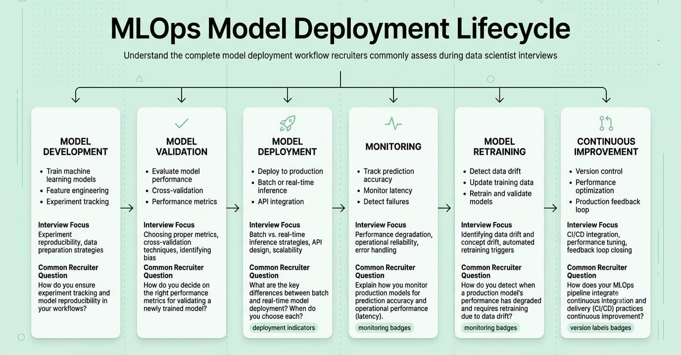
Question 77
Question: What is model drift, and how would you detect and address it in a production model?
Answer: Model drift occurs when a deployed model's performance degrades over time because the statistical properties of incoming data (data/covariate drift) or the underlying relationship between features and the target (concept drift) change from what the model was originally trained on. Detection involves ongoing monitoring of model performance metrics against ground truth (when available), statistical comparison of live feature distributions against the training distribution, and prediction distribution monitoring. Addressing it typically involves scheduled or trigger-based retraining on more recent data.
Explanation: A critical, very commonly tested production ML concept, since a model's real-world value depends entirely on maintaining performance after deployment, not just at the moment of initial launch.
Real-World Example: A demand forecasting model trained on pre-pandemic consumer behavior experienced significant concept drift when the pandemic dramatically and rapidly shifted purchasing patterns, requiring urgent retraining on more recent, representative data to remain accurate.
Common Mistakes: Deploying a model without any ongoing monitoring plan, assuming initial strong validation performance will persist indefinitely without any degradation over time.
Follow-up Questions: What's the difference between data drift and concept drift, and can you give an example of each? How would you decide on an appropriate retraining cadence for a specific model? What would you do if ground-truth labels for calculating live performance metrics are only available with a significant delay?
Question 78
Question: What is the difference between batch and real-time (online) model inference, and how would you decide which a given use case needs?
Answer: Batch inference generates predictions for a large set of inputs on a scheduled basis (e.g., nightly), storing results for later use, appropriate when predictions don't need to reflect the very latest data and can tolerate some staleness. Real-time/online inference generates predictions on-demand in response to individual requests, typically with strict low-latency requirements, necessary when predictions must reflect the most current available information (like a fraud-detection decision needed within milliseconds of a transaction).
Explanation: A foundational production ML architecture decision, testing practical judgment about matching the serving approach to the actual business latency and freshness requirements.
Real-World Example: A weekly email marketing recommendation model can comfortably use batch inference (predictions generated once, in advance, for the whole user base), while a real-time fraud detection system checking each transaction as it occurs requires online inference with a strict, typically sub-second latency requirement.
Common Mistakes: Defaulting to building complex real-time infrastructure for a use case that doesn't actually require it, unnecessarily increasing system complexity and cost when simpler, cheaper batch inference would suffice.
Follow-up Questions: What infrastructure considerations differ between building a batch versus a real-time inference pipeline? How would you handle a situation where the required features for real-time inference aren't readily available with low enough latency? What is a feature store, and how does it help bridge batch and real-time feature consistency?
Question 79
Question: How would you set up monitoring for a machine learning model in production?
Answer: Monitor multiple layers: system/operational health (latency, error rates, throughput), input data quality and distribution (checking for drift, missing values, or unexpected values compared to training data), prediction distribution (checking for unexpected shifts in the model's output distribution over time), and, where feasible, actual model performance against ground truth labels once they become available (which may be delayed) — combined with alerting thresholds and clear escalation processes when anomalies are detected.
Explanation: A foundational MLOps question testing holistic understanding of what needs to be tracked beyond just the initial offline validation metric, essential for maintaining a reliable production ML system.
Real-World Example: A credit risk model in production might have automated alerts if the proportion of applications flagged as high-risk suddenly spikes well beyond historical norms, prompting investigation even before delayed ground-truth default outcomes become available to directly confirm a performance problem.
Common Mistakes: Only monitoring system-level operational metrics (uptime, latency) without any monitoring of data quality, input distribution, or prediction distribution, missing early warning signs of degrading model performance well before it becomes a larger, more damaging problem.
Follow-up Questions: How would you set appropriate alerting thresholds to balance catching real issues against generating excessive false alarms? How would you monitor model performance for a use case where ground truth labels are delayed by weeks or months? What would you do if you detected a sudden, significant shift in the input feature distribution?
Question 80
Question: What is a feature store, and what problem does it solve?
Answer: A feature store is a centralized system for storing, managing, and serving machine learning features consistently across both model training and real-time inference, solving the common and consequential problem of "training-serving skew" — where features computed differently (even subtly) between the training pipeline and the production serving pipeline cause a model to behave unexpectedly or perform worse than expected once deployed.
Explanation: An increasingly important and commonly tested MLOps concept, especially at organizations building and deploying many models, testing awareness of a subtle but very consequential production ML pitfall.
Real-World Example: A feature computed as "average purchase amount over the last 30 days" might be calculated slightly differently in an offline batch training pipeline versus a real-time serving pipeline (different rounding, different time-zone handling, or a slightly different lookback window) — a feature store helps ensure both pipelines compute this feature identically, preventing subtle production performance degradation.
Common Mistakes: Maintaining entirely separate, independently-implemented feature computation logic for training versus serving pipelines without any shared, single source of truth, creating exactly the kind of subtle training-serving skew risk a feature store is designed to prevent.
Follow-up Questions: How does a feature store typically handle both batch and real-time (streaming) feature computation needs? How would you detect training-serving skew if you didn't have a feature store in place? What are some well-known feature store tools/platforms you're aware of?
Question 81
Question: How would you design an A/B test to validate a new machine learning model before a full production rollout?
Answer: Consider a shadow deployment first (running the new model alongside the current production model on live traffic without acting on its predictions, purely to compare outputs and catch unexpected behavior safely), followed by a proper randomized A/B test allocating a portion of live traffic to the new model and measuring the actual downstream business metric impact (not just an offline validation metric) before a full rollout, with a clear rollback plan if issues arise during the gradual rollout.
Explanation: Tests the ability to connect model evaluation methodology with broader experimentation and safe deployment practices, an important practical skill bridging data science and MLOps responsibilities.
Real-World Example: Before fully replacing a production recommendation model, a company might first run it in shadow mode to confirm its predictions are reasonable and the system is stable, then run a proper A/B test on a subset of live traffic to confirm it actually improves the real downstream business metric (like revenue or engagement), not just an offline proxy metric.
Common Mistakes: Relying solely on strong offline validation metrics to justify a full production rollout without any live testing, missing potential issues (data pipeline bugs, unexpected edge cases, or a mismatch between offline metric improvement and actual downstream business impact) that only become apparent with real production traffic.
Follow-up Questions: How would you decide on an appropriate percentage of traffic to allocate to the new model during the A/B test phase? What would you do if the new model shows a strong offline metric improvement but no significant improvement (or even a regression) in the actual live business metric? How would you design a safe, gradual rollout plan with an appropriate rollback trigger?
Question 82
Question: What is model interpretability, and what techniques would you use to explain a complex "black box" model's predictions?
Answer: Model interpretability refers to the ability to understand and explain why a model produced a specific prediction, important for trust, debugging, regulatory compliance, and fairness auditing. Techniques for complex models include SHAP (SHapley Additive exPlanations, based on cooperative game theory, providing consistent feature attribution for individual predictions), LIME (Local Interpretable Model-agnostic Explanations, approximating a complex model's behavior locally with a simpler, interpretable model), and partial dependence plots (showing a feature's average marginal effect on predictions across the dataset).
Explanation: An increasingly important and commonly tested topic given growing regulatory and business demand for explainable AI, especially in high-stakes domains like credit, healthcare, and hiring.
Real-World Example: A bank using a complex gradient boosting model for loan approval decisions might use SHAP values to explain to a rejected applicant which specific factors most contributed to their application's rejection, both for regulatory compliance (many jurisdictions require this kind of explanation) and internal fairness auditing purposes.
Common Mistakes: Treating interpretability techniques like SHAP or LIME as providing a definitive causal explanation of the model's true internal reasoning, when they actually provide an approximation of feature attribution/influence that should be interpreted with appropriate nuance and caution.
Follow-up Questions: How does SHAP differ from LIME in its underlying approach and guarantees? How would you use these techniques to identify and investigate potential model bias against a protected group? What are the tradeoffs between building an inherently interpretable model versus using a complex model with post-hoc explanation techniques?
Question 83
Question: How would you approach versioning and reproducibility for a machine learning project?
Answer: Version control the code (using Git), track and version the specific dataset(s) used for training (using tools like DVC, or at minimum clear, immutable data snapshots), log experiment configurations, hyperparameters, and resulting metrics for every training run (using an experiment tracking tool like MLflow or Weights & Biases), and version/register trained model artifacts themselves with clear metadata linking each model back to the exact code, data, and configuration that produced it — ensuring any past result can be reliably reproduced and audited.
Explanation: A foundational MLOps practice, increasingly expected of data scientists given the growing maturity of production ML engineering standards, and important for both practical debugging and regulatory/audit purposes.
Real-World Example: When a production model's performance unexpectedly changes, having comprehensive experiment tracking and data versioning allows a team to quickly compare the current model against previous versions and pinpoint exactly what changed (a code update, a new hyperparameter, or a shift in the training data itself) rather than debugging blindly.
Common Mistakes: Tracking only code in version control while treating datasets, hyperparameters, and experiment results as an afterthought, making past experiments difficult or impossible to accurately reproduce or audit later.
Follow-up Questions: What experiment tracking tools have you used, and what was your experience with them? How would you version a large dataset that changes frequently without simply duplicating it in full each time? How would you ensure reproducibility when working with inherently stochastic model training processes (like neural network training with random initialization)?
Question 84
Question: How would you approach a situation where a model performs well in offline evaluation but poorly once deployed to production?
Answer: Systematic investigation: check for training-serving skew (are features computed identically in both training and production serving pipelines?), verify the production data actually matches the characteristics of the training/validation data (checking for unexpected distribution shift), review the offline evaluation methodology itself for potential data leakage that inflated the offline metric artificially, and examine whether the offline evaluation metric genuinely aligns with the real business metric being measured in production.
Explanation: A very practical, frequently tested troubleshooting scenario, since this specific gap between offline and online performance is one of the most common and frustrating real-world production ML problems.
Real-World Example: A model showing excellent offline accuracy but poor live performance might be traced to a subtle bug where a feature was computed using future information during offline training/evaluation (data leakage) that simply isn't available at the actual moment of real-time prediction in production.
Common Mistakes: Assuming the production infrastructure itself must be broken as the first hypothesis, without first carefully re-examining the offline evaluation methodology for potential leakage or an inappropriate metric choice that may not actually reflect real-world performance.
Follow-up Questions: How would you systematically rule out data leakage as the cause of an offline-online performance gap? How would you specifically check for training-serving feature skew? What would you do if you confirmed the production data has genuinely, legitimately drifted from the original training data's characteristics?
Part 9: Case Studies & Business/Stakeholder Scenarios
Question 85
Question: How would you approach a case study question like: "Design a machine learning system to detect fraudulent transactions"?
Answer: Structured approach: clarify the business context and constraints (acceptable latency, cost of false positives versus false negatives, available labeled data), define the problem framing (typically binary classification, often with significant class imbalance), propose relevant features (transaction attributes, historical user behavior patterns, device/location signals), select an appropriate model family (often gradient boosting for structured/tabular fraud data, given its strong performance and reasonable interpretability), define evaluation metrics appropriate for the imbalanced, cost-sensitive nature of fraud (precision/recall at a specific operating threshold, cost-weighted metrics), and address deployment considerations (real-time latency requirements, a feedback loop for continuously incorporating newly confirmed fraud/non-fraud labels).
Explanation: One of the most commonly asked open-ended system design case studies for data scientist roles, testing end-to-end thinking across the entire ML problem lifecycle, not just isolated modeling technique knowledge.
Real-World Example: Real production fraud detection systems typically combine a real-time machine learning model with rule-based guardrails (for known, well-established fraud patterns) and a human review queue for borderline, uncertain cases — a hybrid approach reflecting the genuinely high stakes and cost asymmetry involved.
Common Mistakes: Jumping immediately into model architecture details without first clarifying the business constraints, cost tradeoffs, and specific problem framing that should actually drive those downstream technical decisions.
Follow-up Questions: How would you handle the severe class imbalance inherent to fraud detection? How would you design a feedback loop to continuously improve the model with newly confirmed labels? How would you balance the real-time latency requirement against a more complex, higher-accuracy model?
Question 86
Question: How would you approach a case study question like: "How would you design a recommendation system for an e-commerce platform?"
Answer: Structured approach: clarify the specific business goal (increasing engagement, conversion, or average order value — these can call for different optimization targets), consider the available data and cold-start challenges (for new users or new products with no interaction history), evaluate collaborative filtering approaches (leveraging patterns across many users' behavior) versus content-based approaches (leveraging item/user attributes directly) versus a hybrid approach, and define both offline evaluation metrics (like precision@k or NDCG) and, critically, a plan for online A/B testing to validate the actual live business impact, since strong offline recommendation metrics don't always translate directly to real user behavior improvement.
Explanation: Another very commonly asked open-ended system design case study, testing structured problem decomposition for a canonical, widely-applicable business ML application.
Real-World Example: Major e-commerce platforms typically combine collaborative filtering (for established users/products with sufficient interaction history) with content-based approaches specifically for cold-start scenarios (like a brand-new product with no interaction history yet), often further blended with business-rule-based boosting for strategic priorities like promoting new arrivals or clearing inventory.
Common Mistakes: Not addressing the cold-start problem at all, or relying solely on offline evaluation metrics as sufficient proof of the recommendation system's real-world business value without proposing a live A/B testing validation plan.
Follow-up Questions: How would you specifically address the cold-start problem for new users or new products? How would you balance recommendation relevance against beneficial diversity/serendipity in the results shown to users? How would you evaluate whether the recommendation system is creating an unhealthy filter bubble effect over time?
Question 87
Question: A stakeholder asks you to build a model to predict which customers are "high-value," but the definition of "high-value" is ambiguous. How do you proceed?
Answer: Engage the stakeholder in a clarifying conversation to understand the underlying business decision the model needs to inform (is "high value" about current revenue, predicted future lifetime value, or strategic/referral value?), propose a specific, concrete, measurable definition based on that clarified business objective, and validate the proposed definition with the stakeholder and, ideally, relevant historical data before investing significant effort in building the full model.
Explanation: A very common, realistic scenario testing the crucial skill of translating an ambiguous business request into a well-defined, technically tractable problem — a key differentiator between a technically skilled data scientist and one who also delivers genuinely useful, well-targeted business value.
Real-World Example: "High-value customer" could reasonably mean current total spend, predicted customer lifetime value, purchase frequency, or even non-monetary factors like brand advocacy/referral behavior — building a model around the wrong specific definition, however technically well-executed, could produce a fundamentally misaligned and unhelpful result for the actual underlying business need.
Common Mistakes: Making an unstated, arbitrary definitional assumption without confirming it with the stakeholder first, potentially investing significant effort building a technically sound model that ultimately doesn't actually address the real underlying business question.
Follow-up Questions: How would you handle a situation where different stakeholders have genuinely conflicting definitions of "high-value"? How would you validate that your proposed definition actually captures what the business cares about? How would you communicate the tradeoffs of different possible definitions to help the stakeholder make an informed choice?
Question 88
Question: How would you explain a complex machine learning model and its predictions to a non-technical executive stakeholder?
Answer: Lead with the business impact and bottom-line recommendation rather than technical model details, use plain-language analogies to convey the model's general approach (avoiding jargon like "gradient boosting" or "hyperparameters"), focus on what actually drives the model's key predictions in intuitive business terms (using an interpretability technique like SHAP translated into accessible language, rather than raw technical output), and proactively and honestly address the model's limitations and appropriate level of trust/confidence rather than overselling its precision or certainty.
Explanation: A very commonly tested communication question, since translating complex technical work into accessible, actionable business language is one of the most important and frequently underdeveloped skills for data scientists.
Real-World Example: Rather than presenting a churn model's SHAP feature importance plot directly to an executive, an effective explanation might say "the model finds that customers who haven't logged in within the last two weeks and have reduced their usage significantly are the strongest signals of upcoming churn" — translating the technical finding into a clear, actionable business narrative.
Common Mistakes: Presenting dense technical detail (algorithm architecture, hyperparameter choices, raw evaluation metrics) without translating it into business-relevant language and implications, risking the stakeholder disengaging or misunderstanding the model's actual capabilities and limitations.
Follow-up Questions: How would you handle a stakeholder who wants a more technical, detailed explanation than you initially provided? How would you communicate a model's uncertainty or potential for error to a stakeholder used to more deterministic reporting? Can you give an example of a technical concept you've successfully explained to a non-technical audience?
Question 89
Question: Tell me about a time you had to decide between a simpler, more interpretable model and a more complex, higher-performing "black box" model.
Answer: A strong answer describes weighing the specific business context's requirements — regulatory/compliance needs for explainability, the stakes and reversibility of decisions the model informs, the actual magnitude of the performance difference between the simpler and more complex options, and the team's ongoing ability to maintain and debug the chosen approach — rather than automatically defaulting to either "always choose maximum interpretability" or "always choose maximum performance."
Explanation: A common behavioral/scenario question testing practical judgment about a very real and frequent tradeoff in applied data science work, beyond pure technical execution.
Real-World Example: A candidate might describe choosing a more interpretable logistic regression model over a marginally higher-performing but much harder to explain neural network for a credit decisioning use case specifically because of regulatory requirements mandating clear, auditable explanations for adverse decisions.
Common Mistakes: Describing a decision made purely based on personal preference or technical interest, without connecting the choice to the specific, concrete business context and requirements that should genuinely drive this kind of tradeoff decision.
Follow-up Questions: How did you quantify or communicate the performance difference between the two options to relevant stakeholders? What would have changed your decision in the other direction, toward the more complex model? How do you generally approach explaining this tradeoff to stakeholders who might not initially understand why you wouldn't simply choose the "best" performing model?
Question 90
Question: Describe a time a machine learning project you worked on didn't succeed or deliver the expected business value. What did you learn?
Answer: A strong answer honestly owns what went wrong (without excessive self-blame or entirely deflecting responsibility onto others), clearly diagnoses the actual root cause (which might be a poor problem framing, insufficient/inappropriate data, a mismatch between the offline metric and true business impact, or a failure in the deployment/adoption process rather than a purely modeling issue), and articulates concrete, specific lessons genuinely applied to subsequent projects.
Explanation: Tests self-awareness, honest accountability, and growth mindset — since not every data science project succeeds, and how a candidate reflects on and learns from failure is highly revealing.
Real-World Example: A candidate might describe building a technically strong model that was ultimately never adopted because it didn't integrate well into stakeholders' actual decision-making workflow, leading to a subsequent change in process to involve stakeholders much earlier and more continuously in defining requirements and reviewing intermediate results before finalizing future projects.
Common Mistakes: Choosing an example that isn't a genuine failure (a humblebrag), or attributing the failure entirely to external factors without any genuine personal reflection or resulting change in approach.
Follow-up Questions: What would you do differently if you approached that same project again today? How did you communicate the project's shortfall to relevant stakeholders? How has this experience specifically changed your approach to scoping or executing similar projects since?
Question 91
Question: How would you prioritize between multiple competing data science project requests when you have limited bandwidth?
Answer: Prioritize based on a combination of expected business impact (both magnitude and confidence in that impact), feasibility (data availability, technical complexity, and realistic timeline), strategic alignment with current organizational priorities, and urgency — while communicating the prioritization rationale transparently to all requesting stakeholders rather than silently deciding, and periodically revisiting the prioritization as new information or requests emerge.
Explanation: A common time-management and stakeholder-management scenario, testing judgment and communication skill under the very common reality of competing demands exceeding available capacity.
Real-World Example: A well-scoped, high-confidence project with clear, significant business impact and readily available data would typically be prioritized over a more speculative, exploratory project with unclear data availability and less certain business value, but transparently communicating this reasoning to the deprioritized project's stakeholder helps maintain trust and alignment.
Common Mistakes: Prioritizing purely based on which stakeholder is most senior or most persistent, rather than a more objective, transparent framework balancing genuine expected impact against feasibility.
Follow-up Questions: How would you handle two projects with roughly equal estimated business impact but very different technical feasibility or timelines? How do you communicate a deprioritization decision to a stakeholder who's disappointed by it? How do you build in appropriate capacity for unplanned, urgent requests while still making progress on planned strategic work?
Question 92
Question: How would you approach a business problem where leadership wants a machine learning solution, but you believe a much simpler analytical or rule-based approach would work just as well or better?
Answer: Present a clear, evidence-based comparison of the simpler approach against the proposed complex ML solution, honestly articulating the tradeoffs (development time, maintainability, interpretability, and expected performance difference, if any), and let the stakeholder make an informed decision with a full understanding of both options rather than either silently building the more complex solution they initially requested or unilaterally overriding their stated preference without adequate explanation.
Explanation: Tests both technical judgment (recognizing when complexity isn't actually warranted, a genuinely important and often underappreciated skill) and diplomatic stakeholder communication, since pushing back constructively on a stakeholder's initial technical preference requires real tact and clear evidence.
Real-World Example: A candidate might describe a stakeholder requesting a complex machine learning model for a task where a simple, transparent rule-based heuristic (based on a few clearly interpretable business rules) would achieve comparable performance with dramatically less development time, ongoing maintenance burden, and much greater interpretability and stakeholder trust — successfully making that case with a clear side-by-side comparison.
Common Mistakes: Either building the more complex solution requested without voicing a well-reasoned professional opinion when a simpler approach would clearly serve better, or dismissively overriding the stakeholder's request without providing clear evidence and allowing them to make an informed final decision.
Follow-up Questions: How would you quantify and present the tradeoffs between the simple and complex approaches convincingly? What would you do if the stakeholder still insisted on the more complex solution despite your evidence and recommendation? Can you describe a real situation where you successfully advocated for a simpler solution than what was originally requested?
Part 10: Recent Industry Trends
Question 93
Question: How are large language models (LLMs) changing the practice of data science, and what new skills are becoming important?
Answer: LLMs are increasingly used both as productivity tools (accelerating code writing, exploratory analysis, and documentation) and as core modeling components themselves (via prompt engineering, fine-tuning, or retrieval-augmented generation for tasks like text classification, summarization, or extraction that previously required building bespoke models from scratch) — shifting some data scientist work toward effectively leveraging and evaluating these powerful pretrained foundation models, alongside continued need for traditional ML skills on structured/tabular data where LLMs are often not the best tool.
Explanation: A highly current and increasingly frequently tested trend question, testing whether a candidate has genuine hands-on perspective on how LLMs are reshaping (and, importantly, not entirely replacing) core data science work.
Real-World Example: A task like classifying customer support tickets by topic, which previously might have required building and labeling data for a custom text classification model, can now often be accomplished quickly using a well-prompted LLM directly or fine-tuned on a much smaller labeled dataset than would have been needed for a traditional from-scratch model.
Common Mistakes: Either dismissing LLMs as irrelevant to "real" data science work, or conversely overclaiming that LLMs can now replace all traditional structured-data modeling, without recognizing that gradient boosting and other classical methods often still substantially outperform LLM-based approaches on tabular/structured data problems.
Follow-up Questions: How would you evaluate whether an LLM-based approach or a traditional custom-trained model is more appropriate for a specific task? What are the risks (hallucination, cost, latency) of using an LLM in a production data science pipeline? How do you think core data scientist skill requirements will continue to shift as these tools mature?
Question 94
Question: What is retrieval-augmented generation (RAG), and what problem does it solve?
Answer: RAG combines a large language model with an external retrieval system (typically a vector database of embedded documents), retrieving relevant, up-to-date, or proprietary information at query time and providing it as context to the LLM before generating a response — this addresses the LLM's inherent limitations of a fixed training cutoff date and lack of access to private/proprietary data, and can also help reduce hallucination by grounding responses in retrieved, verifiable source material.
Explanation: A very current and increasingly commonly tested applied AI architecture concept, given the growing prevalence of RAG-based systems in real production applications.
Real-World Example: A company's internal customer support chatbot might use RAG to retrieve relevant sections from the company's own product documentation or support ticket history before generating a response, ensuring answers are grounded in accurate, current, company-specific information rather than relying solely on the LLM's general, potentially outdated or generic training knowledge.
Common Mistakes: Not recognizing the key limitation RAG is specifically designed to address (an LLM's static, general training data versus the need for current, proprietary, or highly specific information), or not knowing the basic components involved (an embedding model, a vector database, and the retrieval-then-generation pipeline).
Follow-up Questions: How would you evaluate the quality of a RAG system's retrieval component specifically, separate from the generation component? What are common failure modes of a RAG system, and how would you address them? How does chunk size for document splitting affect RAG system performance?
Question 95
Question: What is the growing importance of responsible AI and algorithmic fairness, and how would you evaluate a model for potential bias?
Answer: Responsible AI practices involve proactively assessing whether a model's predictions or errors disproportionately and unfairly affect specific protected groups, using fairness metrics (like demographic parity, equalized odds, or predictive parity, each capturing a different, sometimes mutually incompatible, definition of "fairness") to quantify potential disparities, and considering both technical mitigations (like reweighting training data or adjusting decision thresholds per group) and broader process changes (like more diverse and representative training data, or human review for high-stakes decisions).
Explanation: An increasingly important and commonly tested topic given growing regulatory scrutiny (in domains like lending, hiring, and criminal justice) and genuine ethical importance, testing awareness of both the technical and organizational dimensions of this challenge.
Real-World Example: A hiring screening model showing a significantly higher false-negative rate (qualified candidates incorrectly screened out) for a specific demographic group compared to others would represent a fairness concern requiring investigation and potential remediation, regardless of the model's strong aggregate accuracy across the whole population.
Common Mistakes: Assuming that simply removing a protected attribute (like race or gender) from the model's input features is sufficient to ensure fairness, without recognizing that other correlated features (a phenomenon sometimes called "proxy discrimination") can still allow the model to indirectly learn and perpetuate similar biased patterns.
Follow-up Questions: Can you explain why different fairness metrics (like demographic parity versus equalized odds) can be mathematically incompatible with each other, and how you'd decide which is most appropriate for a given context? How would you investigate whether a model is exhibiting proxy discrimination through correlated features? What organizational processes would you recommend to help catch fairness issues before a model reaches production?
Question 96
Question: How is the rise of AutoML and no-code/low-code machine learning tools changing the data scientist role?
Answer: AutoML tools automate significant portions of the traditional modeling pipeline (feature engineering, model selection, hyperparameter tuning), increasingly enabling less specialized users to build reasonably strong baseline models for well-defined, standard problems — shifting a data scientist's distinctive value further toward problem framing, thoughtful feature engineering informed by genuine domain expertise, rigorous evaluation and critical validation of automated results, and handling more complex, nuanced, or novel problems that fall outside the scope of what current automated tools handle well.
Explanation: Tests awareness of an evolving tooling landscape and, importantly, thoughtful judgment about where uniquely human data science expertise remains most valuable and differentiated as automation continues to advance.
Real-World Example: An AutoML tool might quickly produce a strong baseline gradient boosting model for a standard, well-structured churn prediction problem with clean, readily available data, but still requires a skilled data scientist to correctly frame the problem in the first place, engineer genuinely valuable domain-informed features the automated tool wouldn't discover independently, and rigorously validate and critically interpret the automated results before trusting them for a real business decision.
Common Mistakes: Viewing AutoML as an existential threat to the data scientist role rather than as a tool that can accelerate certain routine parts of the workflow, freeing up more time for higher-value strategic and judgment-intensive work.
Follow-up Questions: What are the key limitations of current AutoML tools that still require significant skilled human data scientist involvement? How would you critically validate results produced by an AutoML tool before trusting them for an important business decision? How do you see this trend affecting entry-level data science roles specifically over time?
Question 97
Question: What is the growing emphasis on causal machine learning (as opposed to purely predictive machine learning), and why does this distinction matter?
Answer: Purely predictive machine learning optimizes for accurately predicting an outcome, which is often sufficient for many applications, but doesn't tell you what would happen if you intervened and changed something (like offering a discount) — causal machine learning specifically aims to estimate the causal effect of an intervention or treatment, increasingly important as businesses move beyond simply predicting outcomes toward using models to directly inform and optimize actual decisions and interventions.
Explanation: A growing and increasingly tested area at the intersection of traditional causal inference and modern machine learning, reflecting an important industry shift from purely predictive to more genuinely decision-informing, actionable modeling.
Real-World Example: A purely predictive churn model identifies which customers are likely to churn, but a causal (uplift) model specifically identifies which customers' churn risk would actually be reduced by a targeted retention intervention (like an outreach offer) — since some high-risk customers might churn regardless of intervention, while others might be swayed, and this causal distinction directly determines how to most effectively and efficiently target a limited retention budget.
Common Mistakes: Using a purely predictive model's output (like predicted churn probability) directly to target an intervention, without recognizing this fundamentally conflates "who is likely to churn" with the actually more decision-relevant, distinct causal question of "whose behavior would genuinely be changed by our intervention."
Follow-up Questions: What is uplift modeling, and how does it directly address this specific predictive-versus-causal distinction? How would you validate an uplift/causal model's estimated treatment effects, given that you can't directly observe an individual's counterfactual outcome? What data or experimental design would be needed to properly train a causal/uplift model?
Question 98
Question: How is the growing focus on AI/ML sustainability and computational efficiency affecting how data scientists approach model development?
Answer: Increasing awareness of the significant computational cost, energy consumption, and financial cost of training and serving very large models is driving greater attention to model efficiency: choosing appropriately-sized models rather than defaulting to the largest available option, techniques like model distillation (training a smaller model to mimic a larger one's behavior) and quantization (reducing numerical precision to lower compute/memory needs) to reduce serving costs, and more careful cost-benefit evaluation of whether a marginal performance improvement from a much larger, more expensive model genuinely justifies its increased resource cost.
Explanation: An increasingly relevant and commonly tested trend, especially given the rapidly growing cost and scale of modern large models, testing awareness of practical efficiency considerations beyond pure predictive performance alone.
Real-World Example: A company deploying a customer-facing chatbot might specifically use a smaller, distilled or fine-tuned model rather than a massive general-purpose foundation model for many routine, well-scoped queries, substantially reducing serving costs and latency while maintaining acceptable quality for that specific, narrower use case.
Common Mistakes: Defaulting to the largest, most powerful available model regardless of the actual task's complexity and requirements, without carefully weighing the real-world cost, latency, and environmental impact tradeoffs against the marginal performance benefit for the specific business need at hand.
Follow-up Questions: What is model distillation, and how does it work at a high level? How would you decide whether a smaller, more efficient model is "good enough" for a specific production use case? How do you think about the tradeoff between model performance and computational/environmental cost in your own work?
Question 99
Question: What is the increasing role of multimodal AI (models that combine text, images, audio, and other data types), and how might this affect future data science work?
Answer: Multimodal models can jointly process and reason across multiple data types simultaneously (like understanding an image alongside an accompanying text description), enabling new categories of applications that weren't previously practical with single-modality models, and increasingly serving as flexible, general-purpose foundation models that data scientists can adapt and fine-tune for a wide variety of specific business tasks that span or combine different data types.
Explanation: Tests awareness of an emerging and rapidly advancing frontier in AI capability, relevant to understanding how the toolkit and scope of possible applications available to data scientists continues to expand.
Real-World Example: A retail company might use a multimodal model to automatically generate accurate product descriptions directly from product images, or to power a visual search feature letting customers upload a photo of a desired item and find visually similar products in the catalog — capabilities that previously would have required building and integrating several complex, separate specialized models.
Common Mistakes: Assuming multimodal capabilities are exclusively relevant to specialized computer vision or NLP roles, without recognizing their growing, broader relevance and applicability across many general data science and applied business contexts.
Follow-up Questions: Can you think of a specific business use case where a multimodal approach would provide a meaningful advantage over separate, single-modality models handled independently? What are the particular technical challenges specifically involved in effectively combining and aligning different data modalities within one model? How would you evaluate a multimodal model's performance across each of its different constituent modalities?
Question 100
Question: How do you personally stay current with the rapidly evolving field of data science and machine learning?
Answer: A strong answer describes a concrete, ongoing, and sustainable approach: following relevant research (papers, conference proceedings, or well-curated technical blogs/newsletters), participating in relevant technical communities, hands-on experimentation with new tools and techniques on personal or work side projects, and periodically and critically reassessing whether newly emerging tools/techniques are genuinely worth adopting into regular practice versus representing short-lived hype — reflecting genuine, sustained intellectual engagement rather than a generic, one-time answer.
Explanation: A very common closing question testing genuine intellectual curiosity and professional growth mindset, particularly important in a field that continues to evolve unusually quickly.
Real-World Example: A candidate might describe regularly reading specific technical publications or following particular researchers, combined with periodically implementing and experimenting hands-on with a promising new technique or paper on a personal project specifically to build genuine practical understanding before considering recommending its adoption at work.
Common Mistakes: Giving a vague, generic answer ("I just try to keep up with things") without any specific, concrete examples of resources, communities, or particular recent techniques/tools genuinely learned and evaluated.
Follow-up Questions: What's a specific recent development in the field you've found particularly interesting, and why? Can you name a few specific resources (publications, communities, researchers) you follow regularly? How do you personally decide which emerging trends are worth investing meaningful time to learn deeply versus which are likely more transient hype?
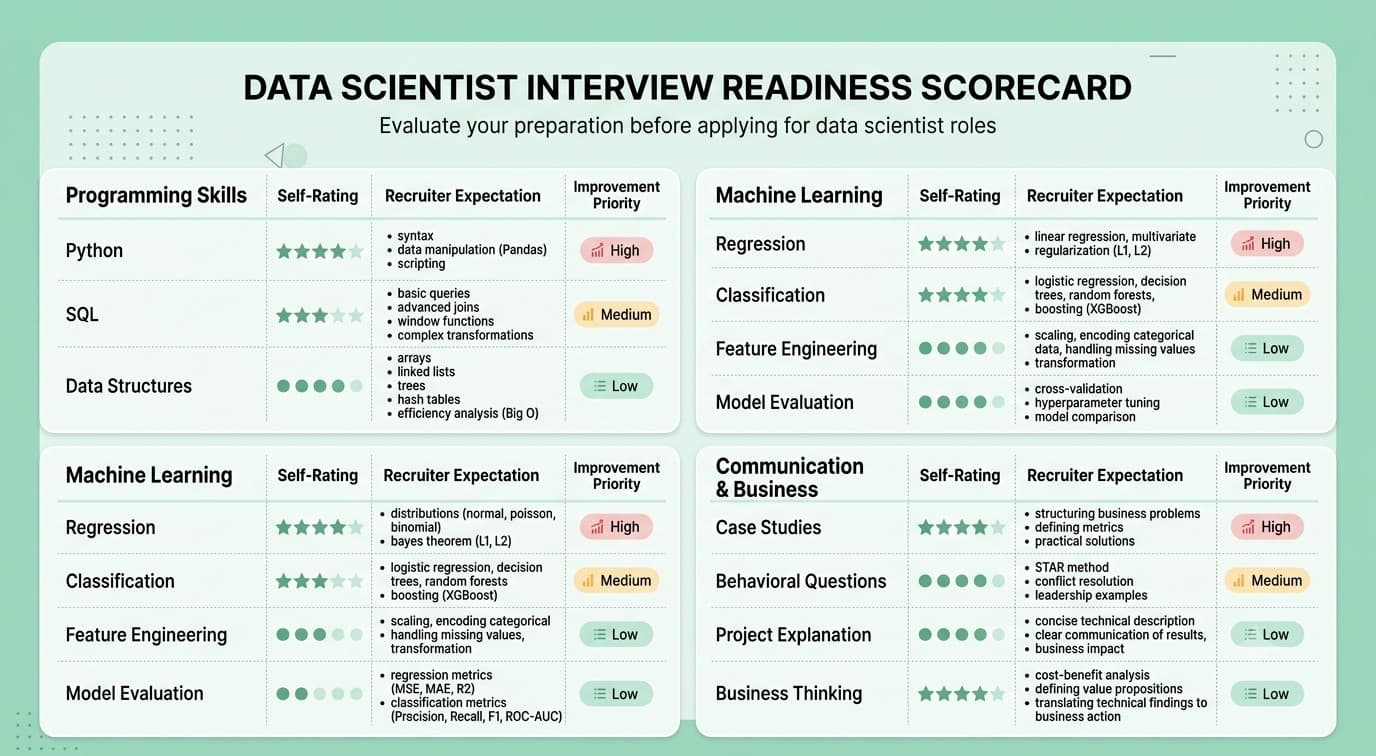
How to Use This Guide
- Don't memorize word-for-word. Use the "Explanation" sections to build genuine understanding, then practice explaining answers in your own words out loud, ideally to another person.
- Prioritize by role emphasis. Research-heavy or applied ML engineering roles should weight Parts 2, 3, and 5 more heavily. Product/growth-focused data science roles should emphasize Parts 7 and 9. Roles at companies with mature ML platforms should focus extra attention on Part 8.
- Practice the SQL and Python questions hands-on. Reading Part 6 isn't enough — actually write and run queries/code against a sample dataset, including edge cases, ideally under mild time pressure to simulate a live technical screen.
- Work through the case studies out loud. For Part 9's open-ended system design questions, practice structuring your answer verbally (clarify, frame the problem, propose an approach, discuss tradeoffs, address evaluation and deployment) since interviewers evaluate your structured thinking process as much as your final answer.
- Prepare your own stories for the behavioral questions. Prepare 5-6 real stories from your own experience that can flexibly answer multiple scenario/behavioral questions throughout this guide, since most such questions are variations on a smaller set of underlying themes (a mistake you made, a disagreement you navigated, an ambiguous problem you structured).
- Use follow-up questions as a self-check. After answering a question, try answering its follow-ups too — this is usually where interviews go deeper and where candidates get caught unprepared.